(B)(N) S&P 100 Volatility Risk and The Full Moon

Indeed, investing is stressful if all we have is hope.

Drama. In this season of volatility and the Full Moon, we are motivated to look at the “Sharpe Ratio” to see if it might help to us to decide on the better risks; the Sharpe Ratio (SR) is a natural consequence of the Capital Assets Pricing Model (CAPM) which we don’t use but it’s the basic feedstock of economists and MBAs and very popular with mutual funds and pension funds; it’s also the staple of the banks’ regulatory capital requirements on a daily basis and why they are so concerned about “volatility” and “market surprise” (Reuters, February 17. 2015, JPMorgan tops list of risky banks: government study).

The Sharpe Ratio is defined as the expected return of an asset above or below a guaranteed risk-free return, such as a government bond, divided by the “volatility” of those returns where, as usual, a return is a percentage price difference between now or later and before – that sounds abstract but that is its most general definition and understanding which we’ll need below; in that form, it’s a measure of investor risk tolerance because two assets with a similar expected return but different volatilities, and therefore uncertainty, are distinguished by the Sharpe Ratio and the asset with less volatility will have a higher Sharpe Ratio and “more return per dollar of (or at) risk” and the common notion is that we need to be paid to take “risks” even though the World would be a dull place and probably die without them.

The word “expectation” is also full of meaning and to think that it might be rendered as an “average” of price returns is a grave error; there are a great many things in investing that the Sharpe Ratio does not and cannot account for because it is driven by price and neither the quality of the asset nor the investor needs for liquidity are wholly accountable to price volatility.

We simplified the calculation but not the principle to SR(asset) = Total ROE/Popoviciu Volatility where the asset is a common stock and the Total ROE is the most recent “investor total return on equity” for the company in the previous year (please see below for further details); the “Popoviciu Volatility” is an upper-bound on the square root of the demonstrated variance for any number of stock prices for the asset that we might take in the corresponding year and it profoundly simplifies to (M-m)/2 where M is the maximum stock price in the course of the year and m is the minimum price, and we can take for the “year” the last 52-weeks which numbers are commonly available and updated daily.

In due course, we invented “The RiskWerk Company Safety Razor” as a cutting-edge tool for bespoke investing using the finest blades for cutting-edge “volatility risk reduction per unit of reward” and what we found is – alas, it is utterly useless because the SR-theory is utterly without foundation despite its good intentions and near universal practice. For those of you who have neither time nor money for failure, please skip to the last section for the “Old Class School” that we used in the NASDAQ 100.

For the rest of us who have the time and money for failure, such as the banks and our pension funds, we need to spend some of it to discover the cause of our failure and that of the Sharpe Ratio (brrrr…so cold).

As Simple As Possible But Not Simpler

We used the word profound to describe the Popoviciu Volatility because that is why it has a name and needed a mathematician (Tiberiu Popoviciu (1906-1975)) to discover it in 1935, more than one hundred years after another mathematician, Johann Carl Friedrich Gauss (1777-1855), discovered mean-variance analysis in 1809 or so, and it lay dormant for nearly 150 years waiting for the investment world to re-discover it and apply it to the stock market which also looked to them like a battlefield in need of ballistics that eventually became statistics and the “Gospel Truth” in the last fifty years or so but they tortured the data and didn’t clear the minefields and victory is in doubt.

Secondly, we don’t know anything about the distribution of stock prices in any time interval (The Tao of Stock Prices (Goetze 2006)) so that a complicated improvement in calculating price volatilities such as something that might depend on their mean or a mean drift or shorter time intervals, is not an improvement at all – prices are just positive numbers for which a stock has been bought and sold by auction at some time and we want an upper-bound on their variance no matter what they are.

If, for example, quarterly results tended to demonstrate some predictable drift in the returns then we could use the quarterly numbers and look at a series of them; in the simpler case in which we don’t suppose that there is a drift or predictable quarterly variation but we want to use the quarterly numbers for earnings and prices, we could use the same formula but since quarterly maximum and minimum prices are not routinely published and the quarterly stock price numbers have no relation to each other quarter over quarter by our assumption, they are statistically independent and carry no memory or recollection of the past or foreboding of the future and the annual variance (V) will be just four times the quarterly variance (VQ) so that 4×VQ = V≤ (M-m)²/4, as above, and hence the Quarterly Volatility = √VQ ≤ (M-m)/4 which reduces the presumed annual volatility by one-half – a constant so that we might as well stick to the annual scenario plus or minus a few basis points.

The Investor Total Return on Equity

Since we’re concerned about returns to the investor, the return on our investment has two parts; one is the dividend yield which is related to the stock price and what we paid for it and the possibility of future payments and capital gains, and the other is our interest, as shareholders, in the increase in the shareholders equity of the company which is increased by the retained earnings, that is, those of its earnings that it doesn’t return to us as dividends but in which we have an interest because we are shareholders and retained earnings might increase or maintain the future value of our investment.

Therefore, the “total return on equity” accounts for both the investor needs for liquidity in so far as dividends are helpful and the price that they’re willing to pay for it by buying and holding the stock and a second part which we call the “market yield on earnings” (please see below) that prices the quality of the asset which tends to be bolstered by the retained earnings that are net of the dividend payment.

Part 1 – The Dividend Yield and The Free Market Ecology

The “dividend yield” is easy to understand and it refers to dividends that the company has paid in the last year and is likely to pay in the next and the current stock prices as if we had just bought them and the company will continue to pay those or similar dividends in the future but the actual dividend yield will be lower or higher for us if we have previously bought the stock at a higher or lower price respectively, and that’s a factor that might moderate the current investor response to changes in the earnings that depends on investor uncertainty and the need for liquidity.

If the company pays a dividend at all, then the “Payout Rate” of the earnings to dividends tends to be about 40% which is a rate that has somehow been discovered by the companies themselves because it’s very close to the Company D modality which is 1/e=0.386 or 38.6% where (e) is the exponential, and it represents a subsistence economy; that is, one which is living hand-to-mouth but can keep-on living indefinitely, and that would be the company which has a disposable income that it can afford to give to the shareholders to feed them and to maintain their interest and not “withdraw” their money by selling the stock and possibly creating downwards pressure on the stock price, perhaps enough to make the company a takeover candidate and somebody else’s lunch.

Figure 1: The Free Market Ecology

We would also expect that an economy would provide us with an income that we might spend it and the economy in this context is an ecology that is formed between the company and its trading connections which include the shareholders and bondholders but not its customers and suppliers and so forth that are essential to the company’s modality which could be quite different from the modality of the company’s payout rate; please see Figure 1 on the right (and click on it to make it larger as required) for examples of the aggregate payout rates in the various major markets.

The retained earnings, however, are at least partially an intangible because they could be burdened with future liabilities as, for example, the depreciation expense account which provides an immediate tax benefit to the earnings, and we don’t know whether the retained earnings that we, as shareholders and investors, have left with the company will pay-off for us in the future because we can normally only benefit from future dividends that are optionally paid by the company and increases in the stock price that are optionally paid by other investors who might not have any money to spare.

Part 2 – The Market Yield on Earnings

The “price to earnings ratio” [P/E] is a stock price-related measure of our confidence in the company to make its earnings and its inverse can be thought of as the “market yield on earnings”; for example, if the [P/E] is 20×, then its inverse is 5% and we can say, for example, that a $5 “coupon” realized as earnings is required in order to support the $100 price of the stock which we know that the market has assigned as a result of the demonstrated [P/E]-ratio.

[P/E]s are never calculated if the earnings are negative but the inverse has a meaning as a charge to the retained earnings or the debt with the “percentage” interpretation of paying or allowing a premium so that, as in the example above in the case of negative earnings, we’re willing to pay $105 for $100 of the equity which is something that we might have to do in order to obtain an income in a deflationary economy because the price of an income tends to be high.

For example, investors are currently holding the stock of the Amazon Corporation for $175.2 billion and that company doesn’t pay a dividend and lost $242 million last year; the “market yield” is -0.242/175.2 = -0.138% or minus 13.8 basis points which is a premium.

Amazon, however, has a net worth of $10.3 billion so what are we to say about a company such as American Apparel Incorporated which doesn’t pay a dividend; has a net worth of minus ($53.7 million); lost ($78.7 million) last year but still has a market value of $154 million? The “market yield on earnings” is minus (51.1%) but because the investors are willing to buy and the hold the stock at $154 million against a debt of $385 million, should we presume that they like the company because it has a negative net worth and is losing even more money?

It’s possible but the normative answer is no and because there are even more egregious cases, we cap the loss at 100% basically writing-off the entire market value and shareholders equity which, of course, is true in fact because the bondholders cannot enforce payment from the shareholders in the event of a bankruptcy but the shareholders can lose all of their investment.

The RiskWerk Company Safety Razor & The Razor’s Edge

We’re all done except for the final step which is to subtract the “risk-free rate” from the “investor total return on equity”, as calculated above, but that rate is not hypothetical or attached to a government bond because it is given to us by the very market that we’re in as the market capitalization weighted average of the investor total return on equity adjusted for volatility and, therefore, adjusted for all of the factors of return that are subject to company or investor discretion as demonstrated by their willingness to pay for them.

For example, the “risk-free rate” that is implied by the behavior of investors in the S&P 100 companies is 0.705% or 70.5 basis points today and it adjusts itself as the market prices for stocks and other investment factors change.

Moreover, it’s not a surprise that the “risk-free rate” means different things to different investors who do not all have the same attitude towards risk or the same money to spend on it (liquidity) and we should not think that the returns on “risk-free” government bonds are in fact “risk-free” because the government can affect the worth of its money by “printing it” and the “risk-free rate” is normally influenced by an auction of government debt among the central and regulatory banks which is further influenced by the need for money, both their own need to lend or borrow and that of the economy and its demand for money.

Hence, we’re better-off understanding the “risk-free rate” by knowing what the investors are willing to pay for it because it is they who will eventually decide its worth and pay its price for better or worse – we don’t need to wait for the Central Bank or the Fed – we already know the answer but they might do something else for which we already know the consequences.

Figure 2: Why is it risk-free?

For example, the current Federal Funds Rate is 0.25% or 25 basis points and the market has been waiting for over a year that it should increase by 50 basis points to 75 basis points when in fact the current “risk-free rate” which the market has defined in the S&P 100 is already 70.5 basis points and a magnificent 80.7 basis points in the entire NYSE market but only 50.5 basis points in the NASDAQ 100.

That means that if the Fed raises the return on “risk-free” government bonds to 75 basis points, then the market will either be happy with that return and buy the bonds or do something else to get a better “expected return”; please see Figure 2 on the right for an explanation of why the market determined “risk-free rate” is “risk-free” and for additional examples in other markets which, as we noted above, have their own ecology.

It will also be noted that the “risk-free rate” in the equity markets behaves like a “bond yield” on those assets which are “the bond”; if the market tends to rise (a bull market, for example) and stock prices are rising, the risk-free rate will tend to decline because of increased volatility and decreasing dividend and market yields (as above); and the reverse is true in a bear market – the dividend and market yields will tend to rise and that is further bolstered by decreased volatility in their “prices”.

In other words, the equity market is a bond market even though only about 1/3rd of the World’s assets are engaged in it; the other 2/3rds are the price of government and peace in the World, so to speak.

The Razor’s Edge

The Razor’s Edge is the market capitalization weighted investor risk tolerance (the Safety Razor, as above, and with the “risk-free rate” also calculated according to the weights assigned by the market capitalization) and we can use it to partition the market into “Lower Risk Tolerance Stocks” with a Safety Razor above the Razor’s Edge and “Higher Risk Tolerance Stocks” with a Safety Razor below the Razor’s Edge (naturally).

The effect on the resulting portfolios is antipodal (like a see-saw) and it raises the Razor’s Edge (to 2.556%) and lowers the risk-free rate (to 0.563%) in the lower risk tolerance case and the reverse in the higher risk tolerance case (to -0.165% and 0.731% respectively) which also means that lower risk tolerant investors are accepting a risk-free rate (0.563%) that is 30% below the rate that is acceptable to a higher risk tolerant investor (0.731%) and 25% below the market (0.705%) – all of which are more than what the government is offering today (0.250%) and raising that rate above 0.563%, for example, will act as an incentive for the low risk tolerant investors to move their money from stocks into bonds and if it’s high enough the higher risk tolerant investors will follow and guess what happens to the stock market – but that is not a cause for a recession – the money is moved but it’s not destroyed and no new money is created but the market will panic anyway in the “flight to safety”.

Figure 3: (B)(N) The Razor’s Edge – Low & High Risk Portfolios

And is there volatility? Yes and so what – volatility has nothing to do with making money in the stock market but it has a whole lot to do with losing it if we’re just standing around and watching the needle on the “volta-meter” and waiting for a signal from “the Fed”; please see Figure 3 on the right (and click on it to make it larger as required) for a summary of the returns on the low-risk and high-risk tolerant portfolios and their difference – substantively nil – but the low-risk portfolio demonstrates a higher latent volatility after having been washed for it akin to why our toothpaste always ends-up at the bottom of the tube and we need a longer-throw to get it to the top.

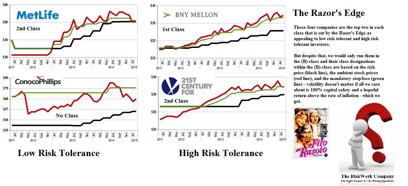
Figure 4: The Ultimate Risk – We can’t help them.

If we iterate that process, we’ll end-up with the one company that provides the greatest incentives to the low risk tolerant investor – Metropolitan Life, right next to ConocoPhillips – and the one company that provides the greatest incentives to the high risk tolerant investor – the Bank of New York Mellon, right next to Twenty-First Century Fox. Oh well.

The S&P 100 1st, 2nd and No Class Companies

Aspern-Essling 1809 and An Unexpected Outcome

Our excursion into the Netherworld brought back the market-determined “risk-free rate” which in this case explains why investors are expecting a hike in the Federal Funds Rate – they’re already working with it.

And although we don’t expect to change investor behavior, we know that the SR-game is no better than a lottery ticket – the market still looks like a battlefield to many investors with a lot of money to move around and once in a while they will be right but they will never understand why?

To play it safe, we need to run the (B)-class portfolio in the S&P 100, and as in the case of the NASDAQ 100, we can partition the portfolio into the 1st, 2nd, and No Class companies to study the ambient effects of “volatility” on the portfolio performance and although there is no reason to avoid any of the classes if we’re managing the portfolio as a (B)-class portfolio, the expected returns are the highest in the 2nd Class, most reliable in the 1st Class, and the lowest in the No Class; please see Exhibit 1 below (and click on it to make it larger as required).

Exhibit 1: S&P 100 Full Moon – Class Stocks

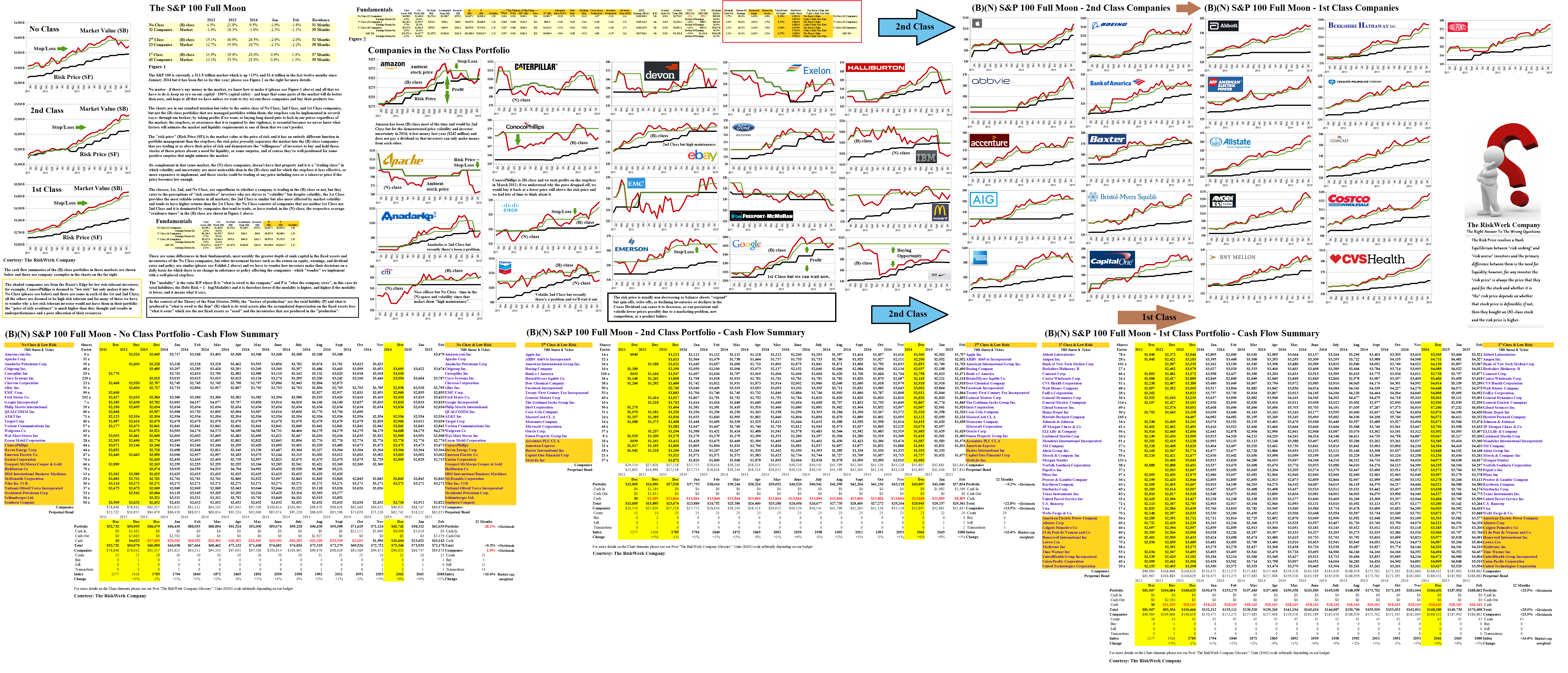
Figure 1.1: (B)(N) S&P 100 Full Moon – Risk Price Chart

For more information on real “risk management” in modern times and additional references to the theory and how to read the charts and tables, please see our Post, The RiskWerk Company Glossary and “(P&I) Dividend Risk and Dividend Yield“, and our recent Posts “(P&I) The Profit Box” and “(P&I) The Process – In The Beginning“; and we’ve also profiled hundreds of companies in these Posts and the Search Box (upper right) might help you to find what you’re looking for, such as “(B)(N) TLM Talisman Energy Incorporated” or “(B)(N) ATHN AthenaHealth Incorporated” or “(B)(N) PETM PetSmart Incorporated“, to name just a few.

And for more applications of these concepts please see our Posts which rely on the Theory of the Firm developed by the author (Goetze 2006) which calibrates The Process to the units of the balance sheet and demonstrates the price of risk as the solution to a Nash Equilibrium between “risk-seeking” and “risk-averse” investors within the demonstrated societal norms of risk aversion and bargaining practice. And for more on The Process, please see our Posts The Food Chain and The Process End-Of-Process.

And for more on what risk averse investing has done for us this year, please see our recent Posts on “(P&I) The Easy (EC) Theory of the Capital Markets” or “(B)(N) The Easy (EC) Theory of the S&P 500“, and the past, The S&P TSX “Hangdog” Market or The Wall Street Put or specialty markets such as The Dow Transports & Utilities or (B)(N) The Woods Are Burning, or for the real class action, La Dolce Vita – Let’s Do Prada! and It’s For You, Dear on the smartphone business.

And for more stocks at high prices, The World’s Most Talked About Stocks or Earnings Don’t Matter – NASDAQ 100. And for more on what’s Working in America, Big Oil, Shopping in America or Banking in America, to name just a few.

Postscript

We are The RiskWerk Company and care not a jot for mutual funds, hedge funds, “alternative investments”, the “risk/reward equation” and every other unprovable artifact of investment lore. We have just one product

The Perpetual Bond™
Alpha-smart with 100% Capital Safety and 100% Liquidity
Guaranteed
With No Fees and No Loads on Capital

For more information on RiskWerk, please follow the Tags or Categories attached to this Letter or simply enter Search for additional references to any term that we have used. Related data may be obtained from us for free in a machine readable format by request to RiskWerk@gmail.com.

Disclaimer

Investing in the bond and stock markets has become a highly regulated and litigious industry but despite that, there remains only one effective rule and that is caveat emptor or “buyer beware”. Nothing that we say should be construed by any person as advice or a recommendation to buy, sell, hold or avoid the common stock or bonds of any public company at any time for any purpose. That is the law and we fully support and respect that law and regulation in every jurisdiction without exception and without qualification to the best of our knowledge and ability. We can only tell you what we do and why we do it or have done it and we know nothing at all about the future or the future of stock prices of any company nor why they are what they are now. The author retains all copyrights to his works in this blog and on this website. The Perpetual Bond®™ is a registered trademark and patented technology of The RiskWerk Company and RiskWerk Limited (“Company”) . The Canada Pension Bond®™ and The Medina Bond®™ are registered trademarks or trademarks of the Company as are the words and phrases “Alpha-smart”, “100% Capital Safety”, “100% Liquidity”, ”price of risk”, “risk price”, and the symbols “(B)”, “(N)” and N*.