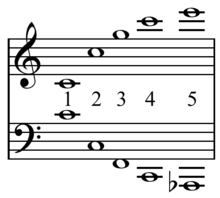
(P&I) The Process
The author gladly and gratefully acknowledges the work of the late
Dr. Verne H. Atrill (1920-1989) who discovered “The Process” and how it works.

The symbol, (a), represents a “process” and the valuation or measure of (a) which we call, a, has values between 0 and 1; small values of “a” near zero indicate the beginning of the process (a) and large values near one indicate the end or completion of the process at a=1. The process (a) is implemented by a process (b) which occurs in the “trading connections” (Coase, 1960) which are required in order to advance or finance the process (a) and the process (b) which receives its “product”.
Both of the processes (a) and (b) can be described in considerable detail in terms of the people and materials that are required to implement the process (a) or (b), but without loss of generality, we think of (a) as a “taking process” which creates “payables” whereas (b) is a “giving process” which creates “receivables” which include the “receipt” of the “product” that is created by the process (a) when the process is complete at a=b=1 and all debts are paid and all receipts are taken.
Moreover, we focus only on payable and receivable events; in general, we don’t assume anything about the actual “production process” and what it does or what materials and skills it might require. Nor do we ever close the books or assume that the future will be anything like the past and cash payments and cash receipts do not close a transaction because there is an enduring economic value in the trading connection.
We can complete this “space” of payables and receivables (net of payments and receipts, which we exclude) and which we can enumerate and call (A) and which consists exactly of the processes (a) and (b) with a σ-algebra that is generated by the subsets of (a) and (b) so that it makes sense to talk about measures and probability; the completion includes all complements and all countable unions of the sets in (A) and, therefore, all countable intersections of the sets in (A) and we can take it to be the smallest σ-algebra that contains all the subsets of (A) (although that’s not material). If n=n(A) is the number of elements in the generators of the completion of (A), which is necessarily finite and which we will also call (A), then we can assign a “probability” of 1/n to each element of the generators of the set (A).
In principle, we can do that today but tomorrow’s answer will be different and our purpose is to understand the process now and what it might be tomorrow based only on what we know now and nothing of its past.
The In-Process Game

The In-Process Game
A 4th Jar Changes Everything
Suppose then that A is a company and that (a) and (b) are the complete process for the company A which consists of every payable (a) or receivable (b) of the company A and its correspondents ab initio, and every payable and receivable of each of these and their correspondents, and so on, although the enumeration eventually terminates (with now) and we generate the σ-algebra over A that we call (A) which contains only what we know and can verify. For example, for every payable, there is a receivable in the books of another company in (A).
Within that set, the sets of all payables (P) and receivables (R) of the company A are measurable and the question is, can the set of payables and receivables of the company A be recovered from the payables and receivables in the complement of that set in (A) which we call (N)?
For example, if the company A has payables (which include its debt, if any) then it also has receivables such as supplies, equipment and fixed plant and the products of its labour, including the development of the “trading connections”.
Moreover, neither payables nor receivables are created “at random” with no purpose. Nor are they created from nothing. Every payable creates a receivable and every receivable creates a payable but by “re-constructing” the payables of A from its receivables, we have “taken it out of the process” as if it were in “bankruptcy” and as if none of the payables will ever to be paid but will need to be settled in what has been left behind. To put it back, we need to recover the “receivables” that are in (b) which is a subset of (N) as above.
If there are k-elements in (b) which we take to be the set of receivables that are due the company A and n-elements in (N) which is the entire σ-algebra except for the two sets (P) and (R) of the payables and receivables of Company A, then the probability of selecting a random receivable in (b) that is due (a) and returning it to (a) is b=k/n. If we do it again, however, the probability is (k-1)/(n-1) which is less than b=k/n; that is, (k-1)/(n-1) = [(k/n) – 1/n]×(n/n-1)= (k/n)(n/n-1) – 1/(n-1)= (k/n)[1+1/(n-1)]-1/(n-1)=(k/n)+[((k/n)- 1)×(1/(n-1))] and the second term is negative if k<n.

We can now play the following “game”: we know that for every payable in the set (P) there is a receivable in (N) and for every receivable in (R) there is a payable in (N); therefore, randomly select an element of (N) and if it is a receivable that corresponds to some payable in (P), mark it as “paid” and put it in (P); if it is a payable that corresponds to some receivable in (R), mark as “received” and put it in (R); if neither, put it back in (N).
If k=p+r is the number of payables in (P) and receivables in (R), respectively, then the outcome is that either one is deducted from both k and n, or neither and both k and n remain the same. As stated, the game only ends in one case, that in which n=p+r so that n decreases by one with every draw. If, however, n>p+r, even by one, the game can never end without violating the independence of each draw from the preceding one. For example, another way to ensure that the game ends is to have a 4th vessel “neither P nor R” so that again n is decreased by one with every draw; however, that procedure establishes a “memory” and violates the independence of the draws.
The best that we can do is to count them and add them up as we get them as R “what is owed to the company” and P “what the company owes” with a probability that is derived from long sequences of no success above observed levels of the count or of P and R.
Although we don’t know what they are, we do know that there are p, r, and n elements in the game and that the probability of “success” in each case is p/n, r/n and (n-p-r)/n for drawing an element of P, R or neither at the beginning of the game.
Suppose then that q=k/n where k=p+r and q is, therefore, the probability of drawing an element in (N) that corresponds to either P or R and we will say “an element of (P) or (R)” even though neither (P) nor (R) are included in (N).
If q=(k-j)/(n-j) is the probability of drawing an element of either (P) or (R) after j such successes, j=0, 1, 2, …, k-1, then the probability of failing to repeat our success (l-1)-times before succeeding on the l-th trial is q×(1-q)^(l-1) and the expected value of such, l=l(j), is [Σl×q×(1-q)^(l-1) : l=1, 2, … any number of times] because we replace the failures and only mark or remove the successes.
However, the expected value of, l, is [Σl×q×(1-q)^(l-1): l=1,2,3,…] = q×[Σl×(1-q)^(l-1)] = q×[-Σ(d/dq)(1-q)^l:l=1,2,3,…] = -q×(1-q)×(d/dq)[Σ(1-q)^l : l=0,1, 2, …]= -q×(1-q)×(d/dq)(1/q) = (1-q)/q = (n-k)/(k-j), j=0, 1, 2,3, …, k-1 and (d/dq) is the usual derivative with respect to q.
The “Game” Plays Music!
And since each game is independent of the last and we need to play the game until j=k (even though we don’t know what k is), we can expect to play the game
(n-k)×[1/k + 1/(k-1) + 1/(k-2) + … + 1]-times = (n-k)×[γ + log(k) + O(1/2k)] for all k but best for k (and n) large enough and where γ=0.57721… is the Euler–Mascheroni Constant (18th century) and “big-O” is big-O (Bachmann–Landau, 19th century).
And to this day (21st century), nobody knows whether γ is a transcendental or even irrational number but it appears regularly in quantum physics and now, in economics and wherever else there is a distinction that might be reconciled by counting.
Informational Entropy Σ(k;n)=(n-k)×[γ + log(k) + O(1/2k)]
This relationship to the “harmonic series”, H(k) = 1 + 1/2 + 1/3 + … + 1/k, gives us pause and it’s called “informational entropy”. The informational entropy of a set with k-elements of which we know nothing is proportional to k×log(k) and demonstrates a state of maximal ignorance or uncertainty in that any of the kˆk subsets of such a set are equally likely and, of course, log(kˆk) = k×log(k) is conspicuous in Σ(k;n) whereas log(n^n)=n×log(n) is not. However, both k and n are in this equation although in different ways. If we put b=k/n so that k=b×n and we can write things like:
Σ(k;n)=(n-k)×[γ + log(k) + O(1/2k)] = ((1-b)/b)×[γ×k + k×log(k) + O(1/2)] and Σ(k;n)=(n-k)×[γ + log(k) + O(1/2k)] = (n-k)×[γ + log(b) + log(n) + O(1/2k)] = (1-b)×[γ×n + n×log(b) + n×log(n) + O(n/2k)] where we note that log(k)=log(b×n).
We also note that the derivative or rate of change of f(k) = [γ×k + k×log(k) + O(1/2)] is f'(k)=γ + 1 + log(k) so that we might expect that Σ(k;n)=((1-b)/b)×f(k) will demonstrate some of the properties of the logarithm function because if b=k/n is more or less constant, then Σ'(k;n) = ((1-b)/b)×f'(k) = ((1-b)/b)×[γ + 1 + log(k)]≈Σ(k;n)/k or Σ(k;n) ≈ k×Σ'(k;n) so that (d/dk) log (Σ(k;n)) ≈ 1/k and Σ(k;n) ≈ log(k) which we already know and, of course, k is an integer and these calculations are “figurative” or “modal” but correct in a neighbourhood of each integer.
The relationship, Σ(k;n)=(n-k)×[γ + log(k) + O(1/2k)], demonstrates that the company A, as “counted” by k, does not expand linearly as k and into “empty space” as (n-k) grows but as log(k) merely because there is a necessary correspondence between payables and receivables and every payable must be matched by a receivable, and vice versa.
Moreover, any counting of transactions, such as k and n, can always be reduced to “counting” in terms of a unit such as the “dollar” or the “penny” so, for example, what counted as one unit of a payable with amount $32.57 counts as 3257 “units” in a much larger space with likely very different probabilities but the same conclusion and, of course, counting them also adds them up.
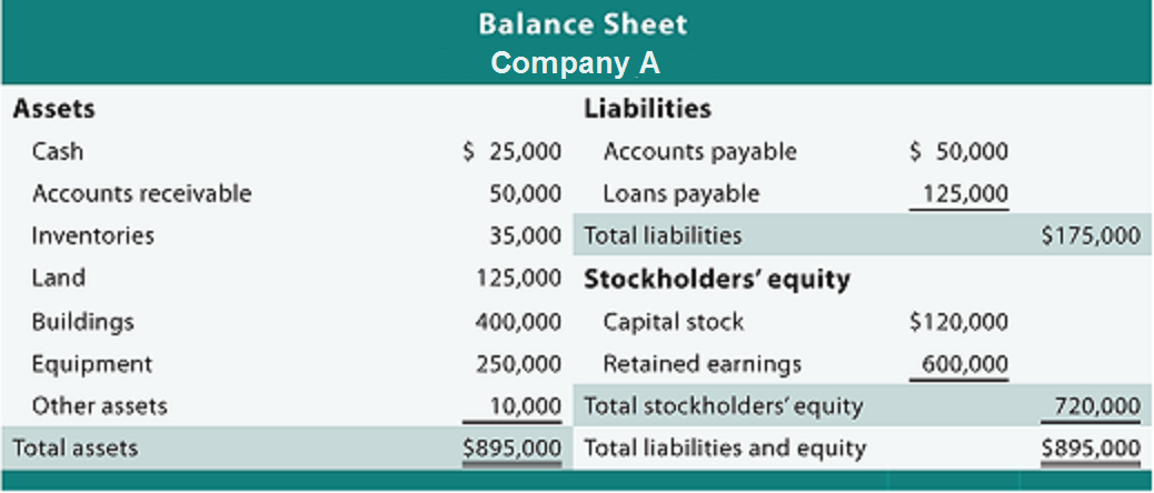
Balance Sheet
Total Assets = Net Worth + Total Liabilities
The company A also has a balance sheet and we would expect that there is a more or less modal relationship between “what it owes” (p) and “what is owed to it” (r); “what it owes” are its total liabilities but what is “owed to it” are the total assets (including cash and near cash or investments) increased by the accumulated depreciation net of “what it owns” which are the inventory and net plant and equipment; the accumulated depreciation is included in “what is owed to it” because it is a real expenditure (and therefore, a receivable) and charge to the net worth and an investment in its own facilities intended to derive future benefits (receivables).
We can therefore express (r) in units of (p) as r = α×p and a “unit” of r is equal to α-units of p (which can itself be expanded into other more basic units related to (N) including α=r/p if we are just counting) and the scale factor, α, is particular to the company A and can be expected to vary from company to company and even within a company over time but if the company is in a “steady state” it should be essentially constant because of the requirement of the balance sheet, Total Assets = Net Worth + Total Liabilities.
If the space (N) were large enough we would expect that the sum of all the receivables (R) should equal the sum of all the payables (P) but that would signify an end to the process in which all receivables were receipts and all payables were payments and R=P and that the system has a very low entropy; in fact, its lowest because there is no uncertainty in the information that we would have about it.
However, the entropy equation, Σ(k;n)=(n-k)×[γ + log(k) + O(1/2k)], which is the same whether we are counting events or counting their value, constrains the system to grow or expand as log(α×P) so that log(R) = log(α×P) and α must be necessarily valued as the average of all the individual α’s belonging to the companies in (N) because we can count events (as above) rather than amounts to get the same effective result.

Figure 1: log(R) and log(P) for the Dow Jones Industrial Companies
For example, with reference to the chart on the right, α = 1.72 ≈ 1/γ where each of the coloured traces is one of the thirty companies in the Dow Jones Industrials over twenty-five quarters (six years) and α is not estimated or posited as 1/γ but calculated as the average of all the observed α’s and reflects, not surprisingly, the interdependence of these companies and their reach into the economy.
If the “system” (which in this example is the Dow Jones Industrial Companies dealing with each other) were to “wind-down” and all the receivables were receipts and all the payables were payments, then, indeed, we would expect that R=P in an “exchange economy”.
But that is not the case when the system is in-process and the issue is, how do we get from stable relationships in a company in which R “what is owed to it” is simply and plausibly related to P “what it owes” as R=α×P to a “systemic” relationship in which log(R) for all the companies is displaced from log(P) for all the companies; or, in other words, “how does the whole become the sum of its parts” (Atrill 1979).
In the above example, the “displacement” is actually quite small; it is log(α)≈log(1/γ)≈0.24 which can be thought of as a percentage difference of 24% from log(R)=log(P) and it is an “excess” that is created by the economy in-process as opposed to an “exchange economy” in which R=P always; and the excess is created by the fact that we have receivables and payables and not just receipts and payments.
And it is in fact the case that, in the above example, R=1.26×P if all the receivables and payables are added up and that is in itself a remarkable result when we consider the 10-fold difference in the actual company α’s which range from α=0.62 for the Home Depot to α=6.26 for the Intel Corporation and around α=1.08 for the banks and financials such as American Express, J.P. Morgan Chase & Company, and Goldman Sachs. We should, however, expect that result whenever (N) is fully developed; it does not necessarily include the “whole world” because payables that are rendered as payments and receivables that are rendered as receipts count for “cash” which doesn’t count and completed transactions which don’t count.

Energy, Mass and Entropy
The Entropy Increases But Mass And Energy Are Conserved And e=(c^2)×m
Suppose then that (a) is a set of payables for company A and that (b) is the corresponding set of receivables that are scattered about in (N) and may belong to one or several companies but which exclude company A.
If a=p((a)) is the probability of the set (a) in (N) and b=p((b)) is the probability of the set (b) in (N), then the entropy (the von Neumann entropy) of each must be conserved as a×log(a) = b×log(b) because each can be discovered by the same independent process (or game) that doesn’t give us any new information because we could use a 4th jar and “discover” k and n more quickly and certainly.
But the process of discovery also requires that the entropy b×log(b) = α×log(a) for the same α=R/P where R is “what is owed to the company” and P is “what the company owes” and “=”-signs in each case can be replaced by “is similar to ≈” and “with probability 1” in respect of the game.
The reason is that when we play the game to discover (b) for (a) we exclude the receivables that belong to company A because they don’t correspond to a payable of company A and we do that without knowledge of what or where they are by accepting either an a or b in (N) when it belongs to (or corresponds to) company A and no other and that result, Σ(k;n), is displaced from log(k) and proportional to k×log(k) or b×log(b) where b=k/n by the constant γ=0.57721… in all cases, regardless of k or n or in which “units” they are counted, in an effectively complete and closed system if large enough.
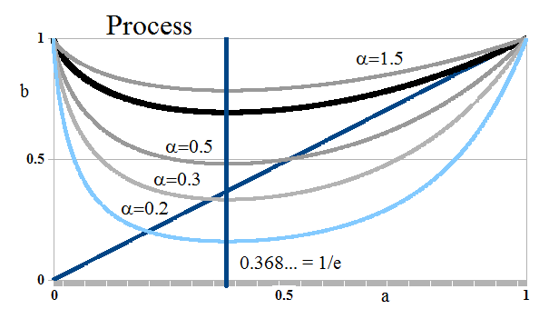
Figure 2: Process With Alpha
The E-Condition a×log(a) = α×log(b)
Similarly, for the same reasons as above, if R is “what is owed to the company” and P is “what the company owes” then the probability b=p((b)) that there is a set of receivables (b) that corresponds to a set of its payables (a) realized with probability a=p((a)), respectively, is similar to b defined by a×log(a) = α×log(b) where α=R/P is the ratio of what is owed to the company (R) by what it owes (P) and we have the two relationships which are both required:
E-Condition: b×log(b) = α×log(a) and a×log(a) = α×log(b) for the same α=R/P.
For example, if P is much larger than R, it is more likely that there is a receivable set (b) that will be assigned to the company with probability b=p((b)) because those to whom the company owes money will have a better chance of receiving it if the company “produces” rather than goes bankrupt; whereas if R is much larger than P, it is less likely that the receivable set with probability b will be assigned to the company because there is less at stake; that is, so much more is owed to the company (R) than what it owes (P) that it would benefit its creditors and trading partners to see it go away. And we note that for any such 0<b<1, p((b)) = b^α tends to one as R/P=α→0 and tends to zero as α→∞.

Niccolò Machiavelli 15th Century
It’s noteworthy, however, that this argument assumes that the company’s creditors will act in their own best interest, having done what they have done and not what they might do in the future if they had a “do over”; if that were not the case, the ratio α=P/R provides the apposite response with equal validity and it’s evident that in realpolitik the “company” which is a government might have quite different objectives than the people that it governs.
To ensure a “positive reciprocity” between the company A and its trading connections, rather than a “predatory” one, the orientation α=R/P has to be same in both cases or the company A would tend to “takeover” its trading connections or vice versa.
The E-condition, then, governs the growth of the firm and its trading connections with respect to each other; the first E-condition, a×log(a) = α×log(b), governs the growth of the firm “into” the trading connections with, basically, increasing “k” with respect to payables in the above notations; and the second E-condition, b×log(b) = α×log(a) governs the growth of the trading connections “into” the firm, again with increasing “k” but with respect to the receivables.
If “k” is not increasing but decreasing, as possibly k→0, so that the firm, company A, is shrinking with respect to its trading connections, then we would expect that if (a) is a subset of its payables, then a=p((a))→0 as (a) shrinks and we can see that the first E-condition remains identically correct as a→0 and b→1. A similar condition obtains if the receivables (b) with respect to company A are shrinking; in that case b=p((b)), which are among the receivables of company A and among the payables of its trading connections, tends to zero and a=p((a)) which is the probability of collecting them, tends to one; if b→0 then a→1 assuming in both cases that the process is “orderly” and in accord with the established order of the E-condition.
However, in order to avoid an explosion by implosion, so to speak, we need to govern “shrinkage” which, of course, happens all the time because firms falter or develop a new set of trading connections for which the old set becomes less relevant.
But as a→0, for example, log(a)→-∞ even as a^a→1, a×log(a)→0 and b→1; which is all good, except for the first, log(a)→-∞; and as we might expect from the in-process game, Σ(k;n)=(n-k)×[γ + log(k) + O(1/2k)] = ((1-b)/b)×[γ×k + k×log(k) + O(1/2)] →+∞ as b=k/n→0 signifying that the company A is becoming much more difficult to “find” or “define” and that the entropy of the system, which is the σ-algebra generated by company A, is increasing.
How The Whole Becomes The Sum Of Its Parts
Energy, Mass and Entropy
The Entropy Increases But Mass And Energy Are Conserved And e=(c^2)×m
Our object now is to “recover” the company A from its parts, its payables and receivables which are scattered about in (N).
If the company A is in-process and displays the modality of the E-conditions with modality α and a=p((a)) is the probability or measure of any subset of its payables, then the least probability or measure b=p((b)) of the corresponding set (b) of receivables in (N) is b such that α×log(b)≥-1/e and the minimum occurs when a=1/e respecting the E-condition a×log(a) = α×log(b). Please see Figure 3 below for an example in the case α=1.
The solution is b=p((b)) such that α×log(b) = -1/e or log(b) = -1/(α×e) so that log(b)→-∞ as α=R/P→0 as long as the firm, company A, or firms exhibiting such process, remain in-process for such modality.

Figure 3: Process With E-Condition Recursion α=1 and all α>1
However, the implication for such (b) in the trading connections is different. The trading connections have the relationship b×log(b) = α×log(a) (which is the reflection of the E-condition in Figure 2 in the diagonal line a=b) and the solution for a=p((a)) is α×log(a”) = b×log(b) and occurs not at a (and by implication, the set (a)) but at a”>a and in the set (a”) for which a”=p((a”))>a=p((a)).
Moreover, α×log(a”)=b×log(b)=(b/α)×(α×log(b)) = (b/α)×(-1/e) = (-1/(α×e))×b =(-1/(α×e))×exp(-1/(α×e)) so that the right-hand side (which defines α×log(a”) in the trading connections) tends to zero as α→0 or gets smaller, much faster (exponentially) than just linearly as in log(b) = -1/(α×e).
We also note that there always two sets, (a(left)) and (a(right)), that are solutions to the first E-condition a×log(a)=α×log(b) with the same b=p((b)) but possibly different sets (b), (b(left)) and (b(right)) for which b=p((b))=p((b(left)))=p((b(right))); and, similarly, the solution (a”) to the second E-condition defines three sets; the set (b) and (b(down)) which satisfy the second E-condition at a” but not the first; and the set (b(up)) which has a’=a” and satisfies the first E-condition but not the second.
In other words, having discovered (a) and (b) in the modality α, the modality is implemented by six sets and defines a “successor” at b→b(up) (b “becomes” b(up), in this context) and a new a→a” (please the upper right-hand corner of Figure 3); and if we iterate the process, then a=a(right) is replaced by a”→1; b is replaced by b(up)→1; and a(left)→0 and b(down)→0.

Figure 4: End of Process With E-Condition a=b=α=1/e
There are also exactly three cases in which nothing happens and there is no “successor” defined by a and b; those are a=b=0 for any α; a=b=1 for any α; and a=b=α=1/e; please see Figure 4 on the right.
We also note, with respect to Figure 3 above, that if we begin with a’ on the left and b(up), then that system “discovers” what we have called “a(left)” and such a(left) will increase to a=1/e and then decrease again as the “system” progresses with a=a(right); moreover, it is at a=1/e that b(up) has its minimum value and b(down) has its maximum value.
If a=1/e, then α×log(b)=-1/e from the first E-condition and the second E-condition defines a” as the solution to b×log(b)=α×log(a”); multiplying both sides by α, -b/e=(α^2)×log(a”) and hence, log(a”)= (-1/e×(α^2))×exp(-1/e×α) and b(down) is defined by b(down)×log(b(down))=α×log(a”)=(-1/e×α)exp(-1/e×α) as we noted above.
Hence, if the process has a modality α and we can discover it, then we know exactly how the process evolves and how it ends as long as there are the required “implementing sets”.
The Company “Alpha”
If (N) is the σ-algebra generated by a “legal” company A, then (N) will, in general, contain many legal companies (and persons) each of which generates the same δ-algebra (N) as company A because of the recursion that we use in its definition.
We also know that for every payable there is a receivable but the only way we know the difference is that we know, for example, that it’s a payable of company A but a receivable of company B because a payable effects a “payment” which is a “receipt” in another company; and a “receivable” effects a “payment” which is for some past service or good that is finally cleared with a “receipt” and a “payment” from another company; we can assume that we know that and play the In-Process Game to discover k=p+r, p and r, for every company in (N) with “probability 1”.
Having done that, we have an array of α’s, one for every company but some of which may be more or less the same; for example, banks tend to show a modality of α=1.08 whereas consumer retail companies tend to show a modality of α=0.8 with seasonal variations, and so forth.
If then (a) is an arbitrary subset of (N), we can say that (a) is a subset of the payables of “Company Alpha” if there is an α and a set (b) with no distinction as to whether it is a set of payables or receivables but will be called a set of receivables of the Company Alpha if a=p((a)) and b=p((b)) are related by the two E-conditions for α; that is, a×log(a) = α×log(b) and b×log(b)=α×log(a) as will (a) also be called a set of the payables of Company Alpha.
That of course is unnerving for an accountant but it is not problem for a mathematician and, in any case, the same solution will yield for the accountants what they want to know. There are, in fact (with reference to Figure 3 and 4 above), only four companies that are interesting in-process; Company A with α<1/e; Company B with 1/e < α ≤ 1; Company C with α>1; and a “Special Company”, Company D with α=1/e.
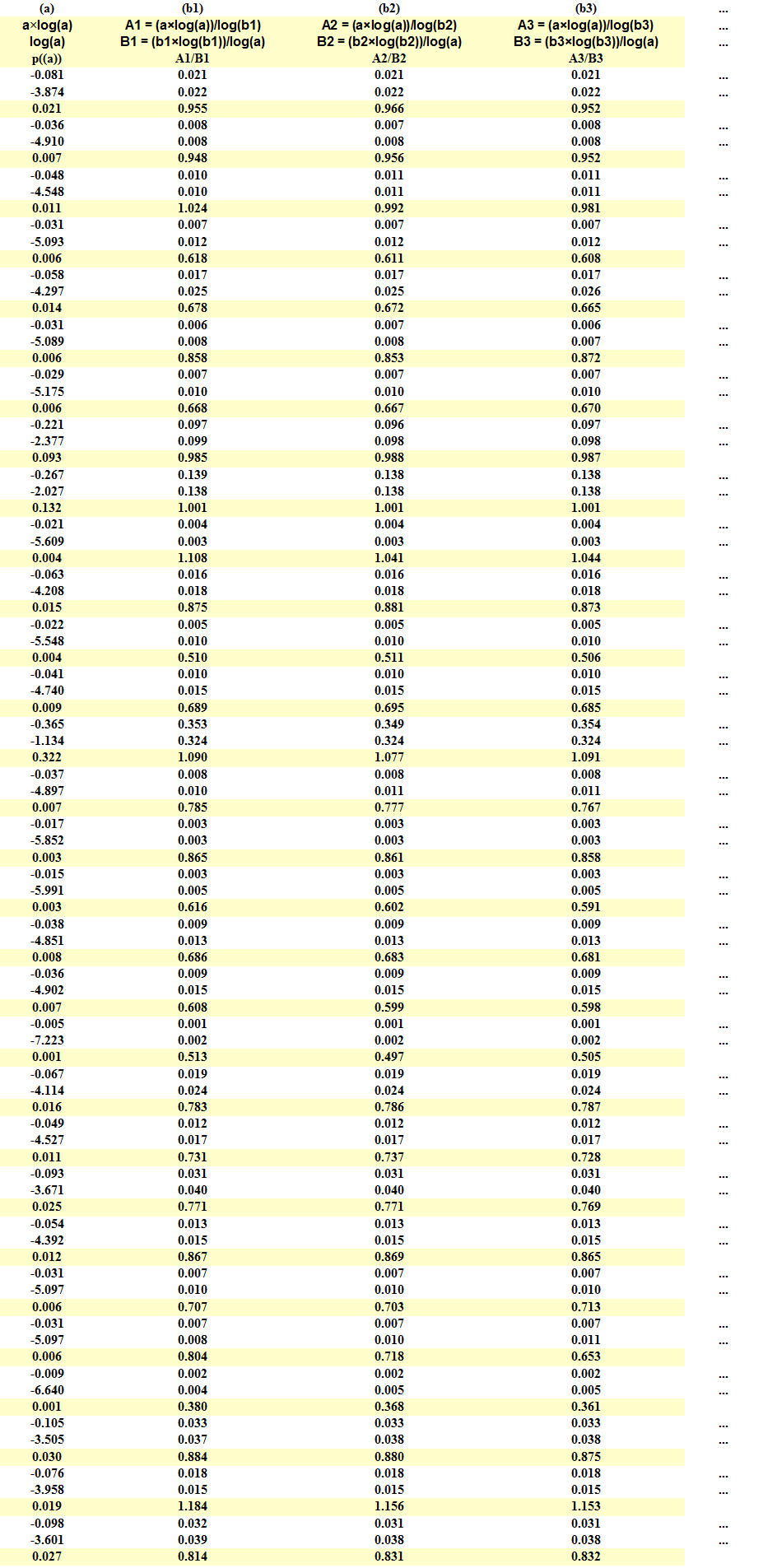
Figure 5: Company “Alpha” A, B, C or D
In fact, we can go one step further. If (a) is an arbitrary set of payables in (N) with measure a=p((a)), we can tabulate all of the subsets of receivables in the complement of (a) in (N) and develop a table with four entries for each such (a) and every (b) which is a subset of (N)\(a) and has a measure b=p((b)): the four numbers are a×log(a), log(b), b×log(b) and log(a) without any presumption of an “α” modality which relates them because we can discover such α if it exists and decide whether any such (a) can be set of payables of one of the four companies, Company A, B, C or D, as above. Please see Figure 5 on the right for an example from the Dow Jones Industrial Companies.
For example, in the first column, we have three rows for the numbers a×log(a), log(a), and their ratio which happens to be a=p((a)) and the measure of the set (a) in (N); in the subsequent columns, which may number in the millions or billions, we have the ratios of the two E-conditions that would relate (a) to (b) and “sample” α’s: (A1,B1), (A2,B2), (A3,B3), and so forth, from subsets of the possible receivables b1=p((b1)), b2=p((b2)), b3=p((b3), and so forth, and their ratios A1/B1, A2/B2, A3/B3, … which if close to one would suggest that such (b)’s may be included in the receivables set that corresponds to (a) with the corresponding α; and that could be done using “statistics”.
If the number of payables is p and the number of receivables in (N) is r, then for each of the (2^p)-subsets of the payables, there are (2^r)-subsets of the receivables to consider and our object is to decide which of these subsets belong to Company A, B, C or D based on their alignment and conformity with the E-conditions.
Company A In-Process

Figure 6: Process With E-Condition Recursion With α = 0.2 and all α< 1/e
If (a) is a subset of the payables in Company A with a=p((a)) and (b) is the corresponding subset of the receivables of Company A with b=p((b)) and demonstrating the modality α which relates them to the E-conditions, then (a) could be either of (a(left)) or (a(right)) which each demonstrate the same α and (b); please see Figure 6 on the right.
Having found such (a) and (b), however, we also find that there may be another (a”) with a(left) < a”=p((a”)) < a(right) which demonstrates the second E-condition (b×log(b) = α×log(a”)) but not the first (a”×log(a”) ≠ α×log(b)) but such (a”) may correspond to the set of receivables ((b(down)) which has a measure b(down)<b and b(down)×log(b(down)) = α×log(a”).
Moreover, there may also be an (a’) (generally two, as illustrated) for which p((a’))= a’ and which satisfies the first E-condition (a’×log(a’) = α×log(b(up)) but not the second for (b) but possibly for (b(up)) with b(up)×log(b(up) = α×log(a”) with a” being smaller than the previous one which satisfies the second E-condition but not the first and is the beginning of the “implementation” in which a becomes a” and b becomes b(up).
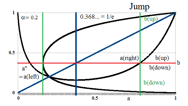
Figure 7: Process With E-Condition Recursion With α = 0.2 and all α< 1/e
However, here we have a problem; if we implement this system with a=a(left) becomes a” with b=b(up) defined by a’ and the first E-condition, the new a” is less than the old a” and we are going “backwards” and will eventually arrive at the maximum extension to the left of the second E-condition which occurs at b=1/e and α×log(a)=-1/e; please see Figure 7 on the right.
In other words, if we think of the process of Company A beginning at a-a(left) and a=p((a)) “small” and there is a set of receivables (b) with p((b))>1/e, then the trading connections “push back” by paying them so that the payables (a) can increase to a(left)=a”, as illustrated, and accumulate so that the process can “jump” from a(left) to a(right) in order to continue its progress to a=1 with the outcome b(up) rather than b(down); otherwise, it’s “stuck” at a<1/e.
For example, if a legal Company A is a gold mine, it needs to start producing and jump from low payables and investment (a receivable) to high payables and production (also a receivable); moreover, if successful, it’s likely to raise its α.
These results suggest (but do not prove) that if a=a(left) then the union of the sets (a)+(a’)+(a”) and (b)+(b(up))+(b(down)) might occur in a successor to (a) in-process; and if a=a(right) then they could have occurred in a predecessor to (a) or still adhere to (a) as p((a)) and p((b)) tend to one. We also note that as (a) increases from (a(left)), (b) decreases and both increase again as (a) approaches a(right) which means, of course, that their measure is increasing in (N).
Moreover, our only requirement for Company A is that the modality α<1/e which allows quite a lot of room for change and adaptation within Company A; if the modality decreases, then both b(down) and b(up) decrease and become nearly equal and it becomes more likely that there is an (a) that includes (a’), (a”), b(up) and b(down) with that modality.
As α→0, both the E-conditions “balloon-out” and approach the boundaries of the rectangle with implications for the “size” of the sets (a) and (b) according to their measures. For example, α=0.1 or less is typical of funding for a new resources mine in Africa or some other remote locale or emerging economy and the debt (or payables) are ten or twenty-times the “receivables” which might not be forthcoming for quite some time.
Our “Company A” could also be a very significant part of the entire economy since governments are usually financed at that level and there are implications of a large (a) such a=p((a)) tends to one in (N) and small or shrinking (b) that eventually becomes one as the creditors band together and overthrow them as, for example, occurred in the French Revolution of 1789.
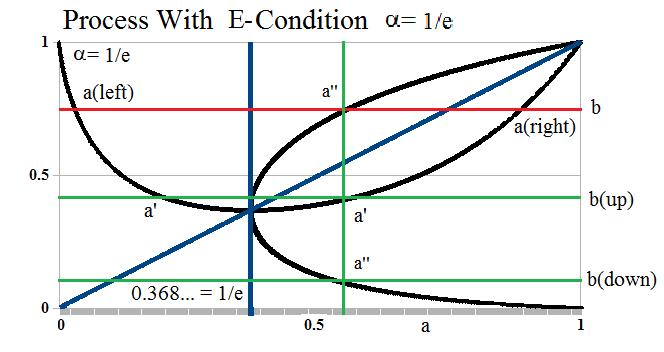
Figure 8: Process With E-Condition Recursion With α = 1/e
On the other hand, the distance between b(up) and b(down) increases as the modality increases to α=1/e and is a maximum at α=1/e suggesting an accommodation to a higher modality as the relationship between payables and receivables changes; please see Figure 8 on the right and note that (a’) and b(up) satisfy the first E-condition (a’×log(a’)=α×log(b(up))) but not the second (b(up)×log(b(up))≠α×log(a’)) but also has an increasing measure in the receivables and the trading connections which might find it helpful to support or adapt to that change.
We also note that the left-most point of the second E-condition always occurs at α×log(a) = -1/e and b=1/e; and for such b=1/e, the corresponding a’ in the first E-condition satisfies the equation a’×log(a’)=α×log(b) = -α; hence a×log(a) = -a/(e×α) = (-1/(e×α))×exp(-1/(e×α)) and a×log(a) < -α = a’×log(a’) for q<α<1/e but the reverse is true for 0 < α ≤q; in other words, Figure 7 in which a'<a is correct only for q<α<1/e; please see Figure 9 and 10 below for α=0.083 < q ≈ 0.1047236…≈ γ/2e where γ is the previously noted Euler–Mascheroni Constant and q is unique; that is, there is one and only one such q.

Figure 9: q-Condition with α = 0.0833
In Figure 9, we have a “firm” that is highly-leveraged and demonstrates the modality α=0.0833 so that the payables are 12× the receivables; if the firm, Company A, is in-process and hopes to complete that process and stay in business, the payables measure a=p((a)) with a=a(left) implies that there is a set of receivables with measure b=p((b)) as illustrated.
In order to advance a, we project that level of receivables to b(up) at a’ which satisfies or conforms to the first E-condition, a’×log(a’)=α×log(b(up)) and also to an a’ which satisfies the second E-condition with a’>a(left) and b(down)×log(b(down))=α×log(a’) but to advance Company A’s process, we need to implement a change from a’ with b(down) on the second E-condition to a” with b(down) on the first E-condition and we note that in order to do that, b(down)<b and it’s also less than b(up).
However, b(up) does not advance Company A’s process because b(up) conforms to the first E-condition with an a” that is less than a’ which we describe as a “q-Condition” and it is the same “jump” to a(right) on b(down) that is required as in Figure 6&7 above but it is a much bigger “jump” and the receivables are less suggesting that the trading connections are receding from this company and to advance it needs to produce more with what it has.
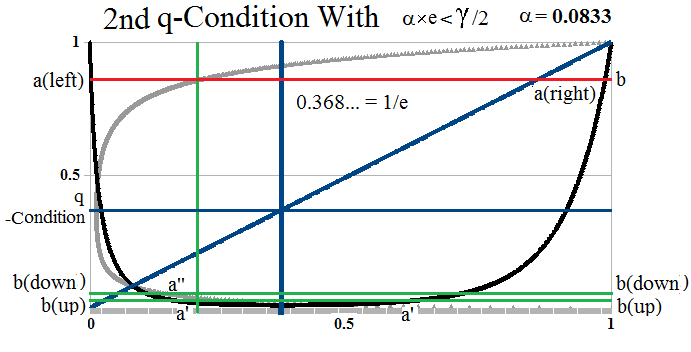
Figure 10: Second q-Condition
We also note that with the same modality a similar situation is obtained with a(left) even smaller and b even more; please see Figure 10 on the right for a sense of “increasing desperation” with the second q-Condition.
In this case, the company has a lower payables at a=a(left) and a higher receivables at b and may have worked its way to a’ at b(up) which satisfies the first E-condition as a’×log(a’) = α×log(b(up)) and, atypically, b(up)<b(down) which satisfies the second E-condition as b(down)×log(b(down))=α×log(a’) but in order to “get” b(down) the company must work its way through payables to a”<a’ and a”×log(a”)=α×log(b(down)) and eventually, a “jump” to a(right).
It’s also worthwhile to remember that some or even all of these sets might not exist but they are required in order for the company to keep or change its modality in a controlled fashion; and if the company is not “random”, it will have a modality.
Extreme Alpha
We noted above that “q” is approximately q ≈ γ/2e ≈ 0.1047236… where γ is the Euler–Mascheroni Constant γ=0.57721… which showed up in the In-Process game. To calculate q, we need to solve the equation q×log(q)=-α and to prove its meaning and uniqueness, that if α×log(a) = -1/e is the solution to the second E-condition with b=1/e and a’×log(a’)=−α is the solution to the first E-condition with b=1/e, then a'<a if α<q and a’>a if q≤α<1/e.
From the two conditions, it follows that a×log(a)=-a/(e×α) and a’×log(a’)=-α and because a×log(a) is strictly decreasing as a function of a as a increases from zero and α≤1/e, we need only show that a’×log(a’)>a×log(a) if α<q and a’×log(a’)≤a×log(a) if q≤α<1/e.
However, a×log(a) – a’×log(a’) = α – a/(e×α) = α +(-1/(e×α))×exp(-1/(e×α)) = α + f(α) with f(α) = (-1/(e×α))×exp(-1/(e×α)) and (d/dα)[α + f(α)] = 1 + [(1/(e×α^2)]×[exp(-1/(e×α))]×[1-1/(e×α)]>0 for all α such that 0<(e×α)<1 and equals zero at α=1/e.; hence α + f(α) is strictly increasing in a neighbourhood of (e×α)<1 and obtains a local maximum at α=1/e but is not necessarily strictly increasing for all 0<(e×α)<1. And, indeed, it isn’t but has only one local minimum for 0<(e×α)<1.
If α + f(α) =0, then log(α) = log(1/(e×α)) – 1/(e×α) and -1 + log(e×α) = -log(e×α) – 1/(e×α) so that log(e×α) = (1-1/(e×α))/2 and we define q = α×e as the solution to the equation log(q) = (1-1/q)/2; then α + f(α) = (q/e) + f(q/e) ≤0 in a neighbourhood of q<1 because q=1 is a solution to α + f(α) =0 ; and α + f(α)>0 if q>1 because α + f(α) is strictly increasing.

Figure 11: Extreme Alpha
However, q=1 is not the only solution to q×log(q) = (q-1)/2 for 0<q≤1; please see Figure 11 on the right.
The solution, q=α×e, satisfies the following result: there are always positive numbers α(k), k=1,2, …. such that Σα(k)=1 and (e/2)[1 – α×e] = Σα(k)/k so that the left-hand side (which is a straight line in α) is always in the convex hull of the harmonic numbers and implies that α ≈ γ/2e ≈0.1047236… as noted above; and with that value of α, Σα(k)/k ≈ 0.967521 whereas if α=γ/2e exactly, then Σα(k)/k = 0.9668822; for the proof, please see the Appendix below.
On the other hand, (e/2)[1 – α×e] = Σα(k)/k = 0 when α=1/e (which is the largest value for q=1=α×e) and it obtains its largest value of e/2 when α=0.
Company B In-Process

Figure 12: Process With E-Condition Recursion α=0.56 and 1/e< α<1
Company B consists of all the payables and receivables in (N) with a demonstrated modality in the range 1/e < α ≤ 1; please see Figure 12 on the right.
In this case, the two E-conditions always have a common solution at 1/e<a=b=α≤1 but the vertical distance between a” near a(right) and a’ and the corresponding b and b(up) shrinks as α increases to α=1 and vanishes at α=1.
As in Company A, we find a(left), a(right), (a”) which satisfies the second E-condition for that modality but not the first; (a’) which satisfies the first E-condition but not the second; and the sets b(up) and b(down) that mediate the E-conditions for a” and a’, respectively.
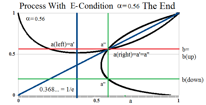
Figure 13: Process With E-Condition α=0.56 and 1/e< α<1 at a=b The End
However, if a=a(left) then the next implementation occurs at a” and b(up) which is substantially to the right of a(left); and if a=a(right), then a” is to the left of a(right) and b(up)<b in both cases.
That process “converges” to the intersection of the two E-conditions at a=b=α by “cycling”; this is, it is a “cyclic process” in which a and b increase and then decrease to a=b as payables work receivables and vice versa; please see Figure 13.

Figure 14: Process With E-Condition α=0.56 and 1/e< α<1 at a=b Jump
But if a(right) is to the left of the point of minimum engagement of the trading connections which occurs at α×log(a)=-1/e, the production may be increasing payables (a) before sales which would increase the receivables (b) and allow a “jump” to the other side; please see Figure 14 on the right.
Moreover, even though both a and b can approach 1, there’s no drive or forcing mechanism in the implementation that would cause them to stay at high levels; the drive is towards “production” and then “sales”; and sales and then more production at a=b=α and the modality can also be thought of as the “wavelength” of the firm and we don’t have any problem in thinking of it as a “cycle” after a “quantum jump” and the same process of “jump” and then production occurs in Company A and is also effected at α×log(a)=-1/e which is the minimum point of “engagement” of the trading connections who are the receivers of product and also the source of financing.
Company C In-Process

Figure 15: Process With E-Condition α=1.5
Company C has modality 1<α<+∞ and for all that, demonstrates a similarity to Company B and is antipodal to Company A; please see Exhibit 15 on the right.
The two E-conditions intersect at a=b=α>1 so that production and sales are not “cyclic” as in the case of Company A, but more “direct” because the Company C is well-financed with payables only a fraction of its receivables as α=R/P>1. Its process starts a high-level of engagement of the trading connections and the company moves quickly from a(left) to a(right) with the usual implementation to b(up). We also notice that b(down) also serves the modality and that the company tends to take in a lot of receivables as well as generate them.
Company D In-Process

Figure 16: Process With E-Condition Recursion α=1/e
Company D has the modality α=1/e; please see Figure 16 on the right. This modality is the beginning of success for Company A and the beginning of a possible failure for Company B and it’s also at this level of financing with roughly 40% debt and 60% shareholders equity that new companies are financed so we might expect that the “implementation” needs to be made and could be either of the modalities for Company A or B.
At this modality, the implementation to a” on the first E-condition from b at a(right) or a(left) leads to a smaller set of payables and a smaller set of receivables at b=b(up) and if the “shrinkage” continues we have a dead-end at a=b=α=1/e; please see Exhibit 17 below.
The Implementation
Everything that we have discovered so far requires only two assumptions: that we can distinguish a brown bean from a black one (which we call the “payables” and the “receivables”); and, secondly, that there is a distinction such that there is a relationship of the form α=r/p which we have called its “modality” even if there is an excess of one over the other which we have described as Company A, B, C and D which is in itself remarkable because we know, in principle, nothing else about these “beans” but have discovered a “jump process” in Company A and a “cycling process” in Company B and a “wealth problem” in Company C and a “death grip” in Company D. any of which can occur while we are counting these beans and “entrap” us, so to speak, in that modality.
Moreover, the process never ends because “the number of ways in which the beans can be distributed but which excludes just two of them (which we didn’t see or “they emitted not enough light” in the modality and units of e/m=c^2) is never the same as the number ways in which the beans can be distributed that includes them both” (Van Quine’s Theorem which is equivalent to Fermat’s Last Theorem).
In the case that R=P and the number of brown and black beans is the same, there will be a strong tendency to successfully separate them in the modality of Company B but that doesn’t happen all at once and any of the other modalities could apply at some stage of the separation.
Figure 17: End of Process With E-Condition α=1/e
The “implementation” is, therefore, similar to the In-Process Game; a company with payables needs to find its receivables; this is, it needs to find its customers and it needs to find its suppliers and it needs to find its employees and establish its process.
A company advances (in the game) by negotiating receivables at b(up) and bringing them in to its own modality (from the 2nd E-condition to the 1st) and the process is cycled between b(up) and b(down) both of which generate payables (a) at the same rate (which we called a’); the trading connections are engaged at b(down) and receivables (b) are moved up to b(up) and eventually to b=1.
We also note that for any modality the minimum engagement of the company with the trading connections is at a=1/e; and similarly, the minimum engagement of the trading connections with the company occurs at b=1/e and posits the lowest level of payables that are of interest to them in the company that is operating at that modality, α.
The process (a) is minimal and exact with respect to the receivables (b) that it is able to generate at that modality and the implementation describes how that is done and how payables and receivables are negotiated and how they are created and resolved; the implementation also allows that receivables may be created at a very high rate if α>1 in Company C and at a very low rate if α<1/e in Company A at all levels of production at that modality.
Such cycling and expansion that is defined by the logarithmic relations of the E-conditions is limited by the possibility of “saturation” in which the highest levels of payables production in-process cannot create more receivables; or, in the language of the game, we cannot “find” them in “finite” time; in business it would be similar to building-up an inventory which we cannot sell other than at a “discount” which changes the production modality; or throwing another slab of metal on a finished car and asking for a higher price.
“Saturation” of the in-process at the process modality, a×log(a) = α×log(b), can be understood as p=p((b))→0 which also implies that a=p((a))→–∞ if the modality is maintained but that’s impossible because we would understand that if b→0, then a→1 from the 2nd E-condition and that the set (a) overwhelms the space (N); moreover, in the case of payables and receivables the extinction of receivables is accomplished by receipts but such extinction also requires that the corresponding payable is extinguished by the delivery of product so that if b→0 we would expect that a→0 as well but that too cannot be accomplished if the modality is maintained because in that case, a×log(a)→0, definitely, and b has the same value as at a=1.
However, the modality constraint can also be described in the equivalent exponential form, a^a = b^α, with a = p/n and b=r/n and it is correct if a→0 or a→1 as b→1 but not as b→0 because the right-hand side tends to zero and reverting again to the logarithmic form that (p/n)×log(p/n) = (p/n)×[log(p) – log(n)] = (1/n)×log(p^p) + (1/n)×log(n^p) = α×log(r/n) = α×log(r) + α×log(n) as r→0 and p→n and n is a constant; multiplying by n on both sides, we have a relation that says log(p^p) + log(n^p) = α×log(r^n) + log(n^n) as p→n and r→0 which is correct for all r, p and n but also suggests that log(n^p) behaves like α×log(r^n) as p→n and r→0 if the modality is maintained.
Hence, it cannot be the case that r→0 as p→n and the formula suggests that n^p behaves like (r/n)^α = b^α as p→n and therefore that n^p behaves like a^a as p→n or that a^a behaves like n^p and therefore p^p as p→n; and r and therefore a cannot tend to zero as b→0 within that modality of which there is always one and the expansion that is implied by p^p cannot occur but is governed by b^α as b→0; and, in fact, p×log(p) is governed by the Stirling Approximation (17th century) as p×log(p) = p + Σlog(k) + O(log(p)) and therefore, log(p) = 1 + (1/p)Σlog(k) + O(log(p)/p) which looks familiar from the game as an average of the outcomes for large n and p.
The other fact that we need to deal with is that the process never ends and that as a→1, then b→1 and there is an exchange in which receivables become receipts, payables become payments, and said receipts are spent and become payables as the payments become receivables again, but mediated by the modality constraint of the 1st E-condition; in effect, we need to subtract 1 from 1=p((N)) to settle the receipts among all the companies in (N) and then subtract it again from 1=p((N)) to settle the payments among all the companies in (N); and at the end of all of that, we still have 1=p((N)) because such subtractions merely re-arrange (N) but don’t extinguish it in the new math of economics.

How All Economies Work by Dr. V.H. Atrill, 1979
The solution to both of these problems was suggested by Dr. V.H. Atrill who proposed that log(a) = lim (1/(b^α)) × log(1+b^α) as b→0 which limit for a = exp(log(a)) is always greater than 2 for 0<a<1 but reduced to a result of 0<a<1 by subtracting 2 (due to the implied exchange at a=b=1) because the limit cannot exceed the exponential e for any α; moreover, the limit respects the relationship between log(p) and the average search times in the game that is required by the Stirling Approximation and any such solution that is based on counting must do that.
Dr. Atrill called this condition the M-condition for the payables and there is a similar condition for the receivables as log(b) = lim (1/(a^α)) × log(1+a^α) as a→0; it’s noteworthy, however, that the limit is not a mathematical limit but a modality because a and b are the probabilities of sets of payables (a) and receivables (b) that are created within the modality α and are required in order to implement that modality and which need to be proven in order to effect the limit.

Figure 18: M-Condition For (a)
The 1st M-condition for (a) is shown in Figure 18 on the right for Company A, B, C and D without taking the limit because “taking the limit” requires an implementation; and in Figure 19 the implication for the receivables set (b) in the case of Company A.
With respect to Figure 18, we note that for sets (a) and (b) for which the modality applies, the maximum extension of (a) into the (b)-space always occurs at a = p((a)) = 1/e for any modality and the meaning of the extension is receivables in excess of what is required to complete the process at a=1 and b=1 where the exchange takes place; in other words, receivables in excess are profit.

Figure 19: M-Condition For (a) And α = 0.2
With respect to Figure 19 and Company A, however, the M-condition for (b) pushes back and the implementation requires that the exchange takes place at b(up) and therefore that a is less than the maximum extension and the profit is less as well.
Company B is similar and shows aspects of companies A and D; only Company D can extract the maximum profit and we noted that that modality is typical of new investments in which there is a 40% equity interest and a 60% debt interest. Company C allows the largest extensions of (a) into (b) but with the least profit.
The chart shows the relative value of “societal profits” in each of the companies A, B, C and D in-process with that modality. The deftly-funded Company A is the relatively most profitable with modality α<1/e if it is able to maintain that modality in-process and is often typical of exploration companies and start-ups; on the other hand, governments are usually funded at that level as well and the chart shows that there is less societal value in the “balanced budget” than in the productive use of debt if the government can remain solvent and not drop into the “Extreme Alpha” which might require an “extreme jump” effected by a currency devaluation or civil unrest.

Figure 20: Kleptocracy
In contrast, Company C is the least relatively profitable even though it might have the most “money” but no sense to invest it in the right places and that modality is typical of under-leveraged investment companies and oil-rich governments and “kleptocracies” that aren’t spending enough to fund profitable development.
Appendix: Extreme Alpha
Figure 11: Extreme Alpha
We need to find the solution of q×log(q) = (q-1)/2 with q=α×e and 0<q≤1; the solution at q=1 is q=1.
The Taylor expansion of log(q) at q=1/e is log(q) = -1 + (eq-1) – (1/2)(eq-1)^2 + (1/3)(eq-1)^3 – … with the signs alternating; however, q<1/e (as may be verified by calculating values of the derivative (d/dq)(q×log(q)) = 1 + log(q) on both sides of 1/e; please see the chart) so that eq-1<0 and we may change the orientation in all the terms but affecting only the odd-powered terms as log(q) = -1 – (1-eq) – (1/2)(1-eq)^2 – (1/3)(1-eq)^3 – (1/4)(1-eq)^4 – ….which also happens to be the Taylor expansion of -1 + log(eq) (as might be expected).
On the other hand, (q-1)/2q = (1-1/q)/2 and 1/q may be expanded in a Taylor series as 1/q = e/eq = e/(1-(1-eq)) = e[1+(1-eq)^1 + (1-eq)^2 + (1-eq)^3 + … ] for eq<1; hence, if log(q) = (q-1)/2q = (1-1/q)/2 for the q that we’re hoping to find, then
(1/2)(1 – e[1+(1-eq)^1 + (1-eq)^2 + (1-eq)^3 + … ]) = -1 – (1-eq) – (1/2)(1-eq)^2 – (1/3)(1-eq)^3 – (1/4)(1-eq)^4 – … .
Let α(k) = ((1-eq)^k)/Σ(1-eq)^k) so that α(k)>0 and Σα(k) = 1; divide both sides of the above equality by Σ=Σ(1-eq)^k and conclude that (1/2)((1/Σ) – e) = -Σα(k)/k where the first 1/Σ = e×q = α×e^2 as above; and hence, (e/2)(1-α×e) = Σα(k)/k and α = (1/e) -(2/e^2)×Σα(k)/k and α is always on a straight line in the convex hull of the harmonic numbers calculated by Σα(k)/k. QED and also note that the solution cannot “bifurcate” further, in which the two E-conditions “interweave”, as α→0 because there are no other such solutions.
Postscript
We are The RiskWerk Company and care not a jot for mutual funds, hedge funds, “alternative investments”, the “risk/reward equation” and every other unprovable artifact of investment lore. We have just one product
The Perpetual Bond™
Alpha-smart with 100% Capital Safety and 100% Liquidity
Guaranteed
With No Fees and No Loads on Capital
For more information on RiskWerk, please follow the Tags or Categories attached to this Letter or simply enter Search for additional references to any term that we have used. Related data may be obtained from us for free in a machine readable format by request to RiskWerk@gmail.com.
Disclaimer
Investing in the bond and stock markets has become a highly regulated and litigious industry but despite that, there remains only one effective rule and that is caveat emptor or “buyer beware”. Nothing that we say should be construed by any person as advice or a recommendation to buy, sell, hold or avoid the common stock or bonds of any public company at any time for any purpose. That is the law and we fully support and respect that law and regulation in every jurisdiction without exception and without qualification to the best of our knowledge and ability. We can only tell you what we do and why we do it or have done it and we know nothing at all about the future or the future of stock prices of any company nor why they are what they are, now. The author retains all copyrights to his works in this blog and on this website. The Perpetual Bond®™ is a registered trademark and patented technology of The RiskWerk Company and RiskWerk Limited (“Company”) . The Canada Pension Bond®™ and The Medina Bond®™ are registered trademarks or trademarks of the Company as are the words and phrases “Alpha-smart”, “100% Capital Safety”, “100% Liquidity”, ”price of risk”, “risk price”, and the symbols “(B)”, “(N)” and N*.
