(P&I) The Theory of the Firm

The Process

Essay. We know that if a firm is in-process and is one of the Companies A, B, C or D of The Process and The Process End-Of-Process then the firm’s payables and receivables will demonstrate the two E-conditions in-process and the M-condition and N-condition at the end-of-process.

In the notation of the process, “in-process” means that if (a) is a subset of its payables (P) with measure a=p((a)) in the σ-algebra (N) generated by the firm and its trading connections, then there will be a subset (b) of its receivables (R) with measure b=p((b)) such that a×log(a)=α×log(b) (1st E-condition) and b×log(b)=α×log(a) (2nd E-condition) and 0<α<+∞ is its modality which is one of Company A (0<α<1/e), Company B (1/e<α≤1), Company C (α>1) and Company D (α=1/e).

That result (Atrill 1979) is in itself astounding because it can be derived by just counting and sorting in the presence of a “Conservation Law” such as the balance sheet, Total Assets = Net Worth + Total Liabilities; or, as another example, the energy and mass conservation implied by the equation e/m=1 in which the unit is defined by c “the speed of light” is one.

Moreover, the M-condition is necessary and sufficient for the “delivery of product” at the “end-of-process” and the N-condition is necessary and sufficient for the “receipt of product” on the “delivery of product” and both such events are realized as a re-arrangement of the sets and their measures in the ο-algebra (N) that results from the conversion of some payables to payments (as cash) and some receivables to receipts in such a way as to preserve the modality of the firm. Please see Figure 1 below

Figure 1: The Process With α=0.2

The M-condition and N-condition are not hypotheses but are consequences of the E-conditions and occur “at the boundary” a=b=1 in the process space or (a)-space of payables and are described as the M-condition log(a) = lim log(1+b^α)/(b^α) as b→0 for the delivery of product and the N-condition log(a) = -1 – lim log(1-b^α)/(b^α) as b→0 for the receipt of product and both such limits occur in the (b)-space of receivables with consequences in the (a)-space of payables.

The modality of a firm in-process is a consequence of its balance sheet, Total Assets = Net Worth + Total Liabilities, which is a “conservation law” and the modality is necessarily calculated as α=R/P where P is “what the firm owes” which is its total liabilities and R is “what is owed to the firm” and it is calculated as its total assets plus its accumulated depreciation less “what it owns” which is its inventory and net plant & equipment (or “fixed assets”); the “inventory” is what is “produced” in-process and the net plant & equipment is what is “consumed” in-process of what it owns both of which are “negotiated” by its payables and receivables which also account for other factors of production such as materials and labour.

The objective of the theory of the firm is to calculate what the firm is “worth” (N*) in-process in the same units as its net worth (N) and therefore in the units of the balance sheet.

The Debit (DB) and Credit (CR) Float

It’s evident that we’ve come a long way from separating beans in jars in the “In-Process Game” to Figure 1 above but at the end of the day, we have to go back there in order to define and understand “profit” and we will also be able to calculate the “balance sheet worth of the trading connections” in the sense of Ronald Coase (1910-2013) which we have called the “Coase Dividend“.

“In order to carry out a market transaction it is necessary to discover who it is that one wishes to deal with, to inform people that one wishes to deal and on what terms, to conduct negotiations leading to a bargain, to draw up the contract, to undertake the inspection needed to make sure that the terms of the contract are being observed, and so on. These operations are often extremely costly, sufficiently costly at any rate to prevent many transactions that would be carried out in a world in which the pricing system worked without cost.” – Ronald H. Coase 1960.

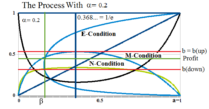
Figure 2: Profit

With reference to Figure 2 on the right which is a Company A with modality α=0.2, we have shown the 1st E-condition (black) which occurs in the process space (or the (a)-space) and the 2nd E-condition (blue) which occurs in the (b)-space of the trading connections but can be represented in the (a)-space as its reflection in the diagonal line a=b which line effectively represents an “exchange economy” in which there is no credit and in which credit is not required so that all payables are payments and all receivables are receipts and the worth of what is paid is exactly equal to the worth of what is received even if, for example, we’re trading edible chickens for inedible gold bars (please see our Post The Food Chain).

The M-condition log(a) = lim log(1+b^α)/(b^α) as b→0 also occurs in the (b)-space but is effective in the (a)-space by first of all subtracting 1 for the delivery of product which effects a transformation of the entire (N)-space because there is a “payment” of payables at a=1=p((a)) and subtracting 1 again for the receipt of product which again effects a transformation of the (N)-space because there is a “receipt” of receivables at b=1=p((b)) and the “end-of-process” occurs at a=b=1 with “probability one” but when we are done, 1=p((N)) as before and always.

The “height” of the M-condition which is measured on the b-axis is the measure of the excess of receivables that are in excess of the delivery of product at a=1 and the receipt of product with a “receipt” of b=1 representing an exact “exchange” of payment for receipt but the Company A will never be able to create the maximum of such excess that occurs at a=1/e and a payables set a=p((a)) with that measure and maintain its modality; the best that Company A can do is determined by the intersection of b=b(up) with the corresponding 2nd E-condition which occurs (in this case with the Company A modality) to the right of the line marked β which occurs at the intersection of the 2nd E-condition and the N-condition (green) and effects the “receipt” of product in contradistinction to its delivery.

Figure 3: Implementing Set in the (a)-space

Hence, at the end-of-process and the delivery of product and the receipt of product, we discover a payables set β=p((β)) and two receivables sets at b=b(down) and at b=profit; moreover, the implementing set b(β) at a=β determined by the 1st E-condition (black) in the (a)-space has yet another value; please see Figure 3 on the right.

The “bottom-line” is, of course, at a=β=p((β)) and b=b(β)=p((b(β))) (which we’ll call the “β-point”) because that is where the process continues after the delivery and receipt of product that occurred at a=b=1; moreover, the process does not start-up again at a=0 but at a=β and as long as Company A maintains that modality, the results will always be the same between the “beginning of process” at a=β to the delivery and receipt of “product” at a=b=1. But we also know that the results depend on the modality and that the results are qualitatively different in the case of Company D “the Death Embrace” at α=1/e and “Extreme Alpha” α < γ/2e ≈ 0.10617… and that the relative position of the M-condition and N-condition changes as the modality increases above α=1/e; please see The Process and The Process End-Of-Process for more details and The Food Chain and The Process Discordant for more examples.

Figure 4: The Working Capital In-Process

The measurable quantities that develop from the process and are conserved as “profit” are the Debit and Credit Float, DB(α) = (1-β)– Arc(β,1) and CR(α) = (1+ (1-β)) – Arc(0,1) where Arc(β,1) is the “length” of the “production line” defined by the 1st E-condition in the (a)-space between a=β and a=1 and Arc(0,1) is the entire length of the process between a=0 and a=1 (Atrill 1979); moreover, we can define the “Working Capital” of the process as W(α) = CR(α) – DB(α); please see Figure 4 on the right.

We’re also going to change our notation in order to emphasize that the quantity 1-β is determined in (b)-space as the “size” of the receivables set that is required to receive the product and we will call that length β so that the Debit and Credit Float are calculated as DB(α) = β– Arc(β,1) and CR(α) = (1+ β) – Arc(0,1) (definition).

Let There Be Light At α=0

The “length” of the “production line” is defined by the In-Process Game and its relevance is assured by the conservation of entropy that is required in that game. And although we don’t show it on the graph in Figure 4, we also know that β→1 (in the new notation) as α→0 (“Extreme Alpha”) so that W(α)→0 as α→0 but W(0)=1 in an extraordinary event that can be described as “lights on” (Genesis 1:3).

In the notation of the game, if (a) is a subset of the payables of Company A, for example, then we need to basically crawl through the entire space (N) in order to match a receivable b∈(b) with every payable a∈(a) but we also know that if the company is in-process then a=p((a)) and b=p((b)) are related by the 1st E-condition a×log(a)=α×log(b); the “paths” are then paths in the Euclidean-space (a)×(N) and we can define a “path-length” as I(α) = Least Upper Bound { ∑ √[ (∆a)² + (∆b)² ]; over all the paths from (a) to (b)} for all such “paths” that we encounter until we are certain “with probability one” that we have discovered (b) for (a); and we know that such upper-bound always exists because the process is finite with probability one.

However, I(α) = Least Upper Bound { ∑ √[ (1+ (∆b/Δa)²]×Δa; over all the paths from (a) to (b)} and this latter is the same as the “line-length” defined by the 1st E-condition in the (a)-space and if one of them exists, so does the other and they are equal; but the latter is easy to calculate simply from the 1st E-condition using the standard calculus even though we don’t make any assumptions about continuity or differentiability.

The “credit float” CR(α) = (1+β) – Arc(0,1) is thus the excess of receivables that are “created” in-process and which is measured by 1+β less the “payables” that are used in-process in order to deliver the product which is Arc(0,1); the “debit float” DB(α) = β – Arc(β,1), however, is always a negative number tending to -1 as α→0 and monotonically increasing to zero as α→+∞; it measures the deficiency of payables in the (b)-space that are required to complete the process and deliver the product and hence, the difference W(α) = CR(α) – DB(α) is the “working capital” in the usual accounting-sense of the current assets less the current liabilities and it depends only on the modality; we also note that β is determined in the “float space” before the delivery and receipt of product whereas the “β-point” is determined after the delivery and receipt of product and will have a value close to 1-β but there is no reason that they should be the same.

The Coase Dividend (GW*)

In order to calculate the “Coase Dividend” (so-named by the author), we need to consider how firms are financed ab initio through a combination of the shareholders equity (N), bond debt (B) and a “working capital loan” (W) which we have called the “N/B/W”-financing model; following Atrill 1979 who broke this ground, the modality of such a firm is defined by α=[N×(1-W)]/1 where, as usual, the numerator is R “what is owed to the firm” and the denominator P=1=B+N is “what the firm owes” and such “1” is more colourfully described as 1=(N(1-W) – M) + B + W where (M) is the “make-up” payment to the bond holders (B) should the firm falter and not come into production; doing the algebra, M=B-B(1-W)=B×W where 1=B+N is the “capital” of the firm.

And we note that the “firm” is not regarded as “owing” the “working capital loan” (W) if the firm is in-process but does pay-back the working capital loan from “what is owed to it” if the firm falters and fails to come in-process with the modality α=[N×(1-W)]/1; in effect, if the firm is in-process, the working capital loan is similar to a “revolving line of credit” and it is never extinguished; moreover, what is owed to the firm in-process is the shareholders equity reduced by the working capital loan (N×(1-W)).

For example, if the investors and bond holders will finance a new company into existence with 40% equity (N) and 60% bond debt (B) and the bank will lend the new company 25% of the “capital” which is 1=N+B in order to bring production on stream (W), then the “N/B/W”-financing model is “40/60/25”, and the modality is α= 0.40 × (1-0.25) = 0.30 which is a Company A modality and just below the Company D modality of α=1/e=0.368… .

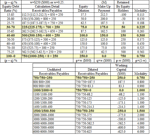
Figure 5: “N/B/W”-Financing Model W=0.25

The “N/B/W”-financing model demonstrates (viscerally) the “societal norms of risk aversion and bargaining practice” by describing what levels of financing investors will provide to a new company.

The “bond debt” (B) is typically regarded as secured by the fixed assets and possibly the inventory (“what the company owns”) whereas the “working capital loan” (W) is a “bank loan” and is regarded as secured by the good faith of the equity owners who will likely pay it back if the firm falters and they intend to do business another day; please see Figure 5 on the right which develops the table of modalities for various financing levels assuming always that the working capital loan is 25% of the capital; the table changes under other assumptions but, as we shall see in the development of the Coase Dividend, the value 25% or 0.25 is virtually mandated by the development of the “float space” in the trading connections; in other words, if we have $100 million in financing by bond debt and equity, we should expect to get $25 million in a line of credit by noon at any bank.

The upper table ends at α=0.75 because the bond debt has disappeared (B=0) and the shareholders are financing the company themselves using their own money and a working capital loan as might be required; if the shareholders can’t get a working capital loan or don’t need one, then they must finance the working capital loan as well and that result is shown in the second table which extends the modality from α=0.75 to any number that we please as long as the shareholders are putting up all of the money and all of which are Company C modalities at α>1 and could be typical of “no credit” or “no credit required”-economies.

If the company does not falter, then it will develop its trading connections and a new modality in-process that is different from the one that it started with and the “balance sheet”  1=(N(1-W) – M) + B + W develops a “new one” 1=1(α) which depends on the modality as 1(α) = (N(α) – M(α)) + B(α) + W(α) with the same meanings as above except that we have absorbed “the diluted shareholders equity” (N×(1-W)) into “the shareholders equity” (N(α)) still allowing for the possibility that the firm might falter in production (bad products or a lawsuit, for example); moreover, the initial condition of the firm is now described in the new unit as 1(α)=(N-M)+B+W and the “bondholders” interest continues to receive the “make-up payment” M(α)=B(α)×W(α) which is now variable (as is the working capital and the bondholders interest) as the “fixed assets” are depreciated and the “inventories” are developed, for example.

However, the modality α=N(α)×(1(α) – W(α)) continues to be described as “the diluted shareholders equity” because the shareholders will need to make good on the working capital W(α) now distributed or “embedded” in the company’s process should the firm falter.

If we substitute M(α)=B(α)×W(α) in the equation of the balance sheet, then 1(α) = B(α) + N(α)/(1(α) – W(α)) and we’ve already shown that the “working capital” as defined above by the modality in-process W(α) = CR(α) – DB(α) has the properties that 0<W(α)<1 and W(α)→0 as α→0 and W(α)→0 as α→+∞ as we might expect; hence, we may define δ(α) = -log(1(α)-W(α)) and δ=δ(α) is a “continuous rate of forward compounding” and 1-δ=1+log(1-W) is a “discount rate” very much as one would “discount” a bond to obtain its present value.

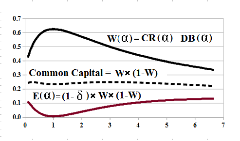
Figure 6: Common Capital and E(α)

The quantity E(α)=(1-δ)×W×(1-W) (with “α” implicit including 1=1(α)) is then the projection of the “common capital” W×(1-W)≈0.25 (please see Figure 6 on the right) which we call the “common capital” because it is “the” amount of money that is deemed to be equally available to the firm or its trading connections as the “working capital loan” without any security (collateral) such as we would require in the bond debt (B).

Since log(1+GW*)=δ, GW* is also the accumulated value of the forward rate of continuous compounding by δ of the “unit” in excess of the unit so that we may equivalence GW* with the result in the float space of the “working” of the “working capital” which is used to develop the trading connections; hence, GW* is the “balance sheet worth” of the trading connections in the float space of the firm and we note that (GW*)=(W)/((1)-W) in the float space.

Are You The One?

If we appear to be “obsessed” by “units”, there’s a good reason for it; in order to evaluate the Coase Dividend in the real values of the balance sheet, we will need to calculate its “float space” in real terms (dollars and cents) and we will need some “new math” in order to simplify the notation and unify the concepts.

The New Math & The Common Capital

The “unit” (1) (with parentheses) is the “firm” and (W) is the “working” of the “working capital” on whatever it is applied to; which means, for example, that (1) + (W)×(1) = ((1) + (W))×(1) is the result of “working” the “working capital” in the firm to create a new payables and receivables “space” which we have called (N); and a “forward accretion” can be represented as (1)/((1)-(W)) = (1) + (1)×(W) + (1)×(W)² + (1)×(W)³ + … whereas “discounting” the present (1) to something previous to the “working” of the “working capital” is represented as ((1) – (W))×(1) so that “discounting” and “forward accretion” are inverses to each other.

Similarly, the “continuous rate of forward compounding” which we have called δ = -log(1-W) is an “operator” on (N) and not just a “scalar”-quantity; and 1-δ=1+log(1-W) which we  have called the “discount rate” is also an operator on the embedding space (N) which returns the “future” to the “present” and we call it the “projection” or the “projection operator”; in particular, projecting an accretion as (1-δ)×(1)/(1-δ)=(1) and returns us to the present.

Hence, GW*=(1-δ)×(W)/(1-W) can be called the “projection” of the discounted “working capital” and the “common capital” (W)×((1)-W) is the “working capital” discounted by the “working capital” and implicitly (W)=(GW*)×((1)-(W)); and (1)+GW*=(1)/((1)-(W)) is the accretion of (1) by the continuous “working” of the “working capital” in (N); we also note that (W) itself is the accretion of the “common capital” as (W) = [(W)×((1)-(W)]/((1)-(W)) so that the “common capital” is a result of the development of the trading connections for the firm and that amount of “currency” in the “float space” is equally attributed or available to both the firm and its trading connections since they are both responsible for its existence because (W) = ((1)-(W))×GW* is the discounted value of now.

In particular, the level of funding (W) in the “N/B/W”-financing model reflects exactly the “demonstrated societal standards of risk aversion and bargaining practice” and the “modal geometry of the firm” (of which basics we have just developed) demonstrates that 〈W〉 ≈ 0.25×(1); please see Figure 6 above. We also note in passing that it is correct to think of the σ-algebra (N) as the “phase space” of the company defined by (P) and (R) (the “sets” of its payables and receivables and those of its trading connections) with “canonical variables” P and R and a “modality” α=R/P which is “conserved” in the familiar terminology of dynamical systems.

The Future Is N*

If Company A is a real firm then we calculate its demonstrated modality as α=R/P where P is “what the firm owes” and is its total liabilities and R is “what is owed to the firm” and is its total assets plus its accumulated depreciation less “what it owns” which is its inventories and fixed assets which are depreciated in production (but we exclude amortization); moreover, the “total liabilities” P are just the complement of the shareholders equity N as Total Assets = N + P.

If we know R and P, then we can “normalize” them as R+P=1 and accordingly, R=α/(1+α) and P=1/(1+α) and the new 1=(1) is the firm on which we “operate” with the “working capital” 〈W〉 in the “float space” (N) that is created by the firm and its trading connections; the future of the shareholders equity (N) in-process is (N*) = (N)/((1)-(W)) as is the future of the firm (1*) = (1))/((1)-(W)); and the “balance sheet” of the future of the firm is (B) + (N)/((1)-(W)) = (1*) (or 1(α) as we’ve previously noted).

In order to “calibrate” the future of the firm with its present, we need to project the “value” of (N*) and (1*) which exist in the “float space” into the real-values of the balance sheet as we know it now by using the “projection operator” (1-δ) which amounts to simply resolving a number of linear equations:

(1.1) (1-δ)×(GW*) = GW* = (R+P)×[(1-δ)×W×(1-W)] where the left-hand side is in the “float space” and the right-hand side is in the real-values or units of R and P as calculated from the balance sheet; and the “factor” E(α) = [(1-δ)×W×(1-W)] is calculated in Figure 4 above;

(1.2) (1-δ)×(1*) = Accumulated Depreciation (Depn) + GW* which we have just calculated and we note that (1*) is the accretion of (1) by ((1)-(W)) which is the “working” of the “working capital” and results in the depreciation of the fixed assets and the creation of GW*; if the firm falters, (1-δ)×(1) = 0;

(1.3) (1-δ)×(B) = -Inventories (Inv) – Net Fixed Assets (Pn) where we note that the “bond debt” in the “float space” does not create float because the bond debt is secured by the net fixed assets and inventories; the “bond debt” like cash has no value in the float space;

Hence, with reference to the “balance sheet” in the float space, (B) + (N*) = (1*),

And that’s all there is to it.

(1.4) (1-δ)×(N*) = N* = Depn + GW* + Inv + Pn is a deduction and necessary consequence of the first three equations.

As an example, suppose that R+P=$1 (one dollar or 100¢) and the modality of the firm is α=R/P=1; then W=0.620 (from Figure 4) and 1-δ = 1+log(1-W) = 0.02449 and E(α)=(1-δ)×W×(1-W)=0.00575; hence:

The “worth” of (W) = (1-δ)×(W) = 1.53¢
The “worth” of the “common capital” (W×(1-W)) = 100×E(α) = 0.58¢
The “worth” of the “firm” (1) = (1-δ)×(1) = 2.45¢
The “worth” of the “shareholders’ equity” ((N)=α/(1-W)) = (1-δ)×(N) = 6.50¢
The “worth” of “what is owed to the firm” (R) = (1-δ)×(α/(1+ α)) = 1.22¢
The “worth” of “what the firm owes” (P) = (1-δ)×(1/(1+ α)) = 1.22¢
The “worth” of the “worked shareholders’ equity” (N*=N/(1-W)) = (1-δ)×(α/(1-W))/(1-W) = 17.23¢
The “worth” of the “Coase Dividend” GW*= (1-δ)×(W/(1-W)) = 4.05¢
The “worth” of the “bond debt” (B = 1 – N/(1-W)) = (1-δ)×(B) = (14.78¢) (negative).

What’s important about these numbers, of course, is their relative size; for example, the firm is worth 6.50¢ today (N) but if it remains in-process, it’s worth 17.23¢ (N*) or more than twice as much; similarly, the Coase Dividend is not insignificant and equal to 4.05¢ which is more than half of the shareholders equity (N) but only a quarter of the future value of the firm (N*) which depends on it; it’s also noteworthy that we only need to know the modality in order to calculate all of these “particulars” of the firm if it remains in-process.

For more applications of these concepts please see our Posts which rely on the Theory of the Firm developed by the author (Goetze 2006) which calibrates The Process to the units of the balance sheet and demonstrates the price of risk as the solution to a Nash Equilibrium between “risk-seeking” and “risk-averse” investors within the demonstrated societal norms of risk aversion and bargaining practice. And for more on The Process, please see our Posts The Food Chain and The Process End-Of-Process.

Postscript

We are The RiskWerk Company and care not a jot for mutual funds, hedge funds, “alternative investments”, the “risk/reward equation” and every other unprovable artifact of investment lore. We have just one product

The Perpetual Bond™
Alpha-smart with 100% Capital Safety and 100% Liquidity
Guaranteed
With No Fees and No Loads on Capital

For more information on RiskWerk, please follow the Tags or Categories attached to this Letter or simply enter Search for additional references to any term that we have used. Related data may be obtained from us for free in a machine readable format by request to RiskWerk@gmail.com.

Disclaimer

Investing in the bond and stock markets has become a highly regulated and litigious industry but despite that, there remains only one effective rule and that is caveat emptor or “buyer beware”. Nothing that we say should be construed by any person as advice or a recommendation to buy, sell, hold or avoid the common stock or bonds of any public company at any time for any purpose. That is the law and we fully support and respect that law and regulation in every jurisdiction without exception and without qualification to the best of our knowledge and ability. We can only tell you what we do and why we do it or have done it and we know nothing at all about the future or the future of stock prices of any company nor why they are what they are, now. The author retains all copyrights to his works in this blog and on this website. The Perpetual Bond®™ is a registered trademark and patented technology of The RiskWerk Company and RiskWerk Limited (“Company”) . The Canada Pension Bond®™ and The Medina Bond®™ are registered trademarks or trademarks of the Company as are the words and phrases “Alpha-smart”, “100% Capital Safety”, “100% Liquidity”, ”price of risk”, “risk price”, and the symbols “(B)”, “(N)” and N*.