(P&I) The One World Food Bank
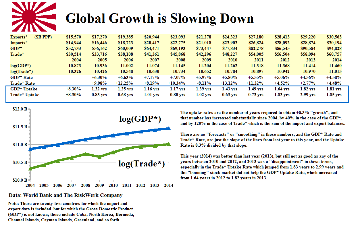
Figure 1: The One World Food Bank
Essay. Inflation and deflation don’t “drive” growth but are side-effects of whether the price of an income, from money, is decreasing (inflation) or increasing (deflation).
For example, if an economy is prosperous and burgeoning, then both business and government will need to borrow money in order to finance the infrastructure – better roads, more labor, better labor, and so forth for the government, and more plants and inventory for the businesses; hence, the rate of interest will tend to rise and provide a “cheaper” income from money (as above), and possibly also better value in stocks if these companies continue to thrive because many investors, and a great deal of money, prefer bonds to stocks, even if the rate of interest on the bonds still falls short of a real return.
With that growth, we can expect “inflation” as a consequence – a higher price for baskets of consumer and producer goods and services – because of the increased demand for them, and more money from incomes to pay for them.
However, that is quite different from just “more money” for which we don’t have a productive use, other than to buy assets which other people might sell if the “price” is high enough and, therefore, the money is cheap as it has been for the last several years in search of an income, and the world economy has been essentially deflationary for the last several years, and even longer, because we need to pay a very high price for an income.
But this distinction also raises the question of whether there are any “deflationary economies” that are growing, or any “inflationary economies” that aren’t, and of course, which economies are growing and which aren’t.

Keynes General Theory 1936
Moreover, the monetary policy decisions of the last few years, since the “recession” of 2008 and 2009, and also post the recession of 2002 and 2003, have promoted a “juvenile” growth-spurt which has since returned to its long-term “deflationary” tendency (please see Figure 1 above), which is alarming because our other “juveniles” are still growing, in number and size, although not as fast as they used to.
Hence, we need to look at the “One World Food Bank” before they start looking at us, or we start looking at each other, because a systemic deflation always results in a declaration of war, and war always results in inflation for the “winners” and hyper-inflation for the “losers”, although, in reality, there are never any “winners” or “losers” in the long term – the “issues” are just deferred to another day.
We also note that “criminal activity” in the black markets, grey markets, corruption, banditry, piracy, crime, and so forth, is deflationary because the proceeds of such crime will pay almost any price for an income; it’s not “inflationary” because the supply of cash from these activities is much greater than the demand for it, and there are more than a dozen countries – all of which are deflationary – for which crime is beyond the reach and control of the government, notwithstanding the government itself.
Moreover, it is not a surprise that economies everywhere tend to be deflationary all of the time; that is, we should always expect downwards pressure on prices, and a high price for an income, whether it be in the cost of acquiring a productive business, or the price of stocks, or just the cost of an education that we might find a job.
The normal end of a deflation, absent a declaration of war, is a recession and a pent-up demand for goods and services that tends to raise their prices, and low prices for an income because there is a demand for money to finance growth in the fixed assets and inventories of businesses.
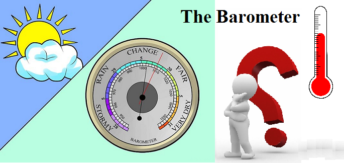
As a result, we’ve developed a “barometer” that can tell us whether we are in a “high pressure” or “low pressure” economic environment which is about to change, and how it might be changed, and which is quite different from the usual measures of “inflation” and “deflation” which just tell us the “temperature”, but not what to do about it; please see below, but before we can do that, we’ll need to make a small excursion into the Theory of the Firm and The Process.

Are you the One that we’re looking for?
Inflation and The Disappearing One
“Growth” in a firm, or government, “enterprise” can always be described by an “operator”, W, that acts on the “factors of production” which are the “fixed assets” at cost, and later, net of the accumulated depreciation, and the “inventories” which are the product or service that is to be sold; and the Coase Dividend, GW*, which becomes an asset of the firm because that is the “factor of production” that activates the fixed assets, the inventories, and the process that produces them, and the customers that buy them, and the suppliers that provide the materials (including labor).
Moreover, the operator, W, can always be discovered no matter at what stage of the development of the firm’s “production process” by re-casting it as an “N/B/W’-financing model in which (N) is the “shareholders equity”, (B) is the “bond debt”, secured more or less by the net plant and equipment, and the inventories, and W is the “working capital”, where we have used quotes around the term because it’s not necessarily the “working capital” that is calculated by the accountants as the current assets less the current liabilities due within one year; our(W)is more enduring and “time” enters into the picture in a different way.
The Theory of the Firm shows that any such “N/B/W”-financing model respects the “demonstrated societal norms of bargaining practice and risk aversion” and results in exactly one parameter, the modality, α=R/P, where (R) is “what is owed to the firm” and (P) is “what the firm owes”, which are its “total liabilities” as calculated from the balance sheet.
“What is owed to the firm” (R) are its total assets plus its accumulated depreciation less “what it owns”, which are its net fixed assets and its inventories (as above).
There isn’t anything else, whether it is a firm or a government, except the Coase Dividend, GW*, which is the result of the success of the firm’s management in developing and sustaining the “production process” and which, ab initio, defines how the “common capital” (please see below) is used to produce the first, W, in a recursive relationship that we cannot resolve without actually knowing the firm’s modality, α=R/P, as above, because one defines the other.
But that’s not a problem because the Theory of Firm shows us what it must be, and how to calculate both the modality and W from the balance sheet.
The “capital” of a firm is the sum of the shareholders equity (N) and the bond debt (B), and we also know (please see below) how to calculate those “quantities” for governments; if the firm does not “come on stream” and “produce” after the investment of the capital in the fixed assets, and the production of inventories or services that can’t be sold, then the capital of the firm, which we’ll call (1), is effectively reduced to (0) by assets that are depreciated and perhaps not wanted by anyone, and inventories that no one wants to buy.
On the other hand, if the firm does come on stream, and creates the viable 〈W〉 as above, then the “growth” of the firm can be described as (1) + 〈W〉 + (W)² + (W)³ + …, and so on, where we think of 〈W〉 as an action or an operator first acting on the “capital”, (1), to “create” 〈W〉, and thereafter, acting only on its “progeny” as 〈W〉 on 〈W〉 = (W)² and 〈W〉 on (W)² = (W)³, and so on, and the “job” of 〈W〉 is to create “payables” and “receivables”, for which the production of a product or service for sale, is incidental and not really of any interest to us – that’s the responsibility of the management, or the government.
As investors (or citizens), we wonder only about what the income will be from our original (1), which is now “owned” by the firm and “in-process”, and we can’t get it back without selling our ownership interest, which might not be worth anything, but we can hope that what the (1) and the 〈W〉 produce, namely 〈W〉 + (W)² + (W)³ + …, and so on, will eventually amount to a (1), which is what we started with, and the return of our (1) is all that we can hope for, although it’s possible that someone will be willing to pay more, or less, for our (1) than (1), and we might have to sell it for liquidity reasons; however, if 〈W〉 is viable, it will produce many (1)’s – we just don’t know when, or how fast.

Figure 2: Traders Almanac – The Profit Box – Company D
The “growth operator” δ = log( (1) + 〈W〉 + (W)² + (W)³ + …), where we have used the parentheses to emphasize that 〈W〉 is not a scalar quantity, but an “operator” that “maps” (1) and its progeny in the “space” of payables and receivables that are created in-process in a well-defined and singular process for which we need only know its modality, α=R/P, which is an invariant for that process, not ruling out the possibility that the process will change over time and establish some other modality, which is done through the “Profit Box” and “random events” that are out-of-process and of measure zero; please see the illustration in Figure 2 on the right and our Post “(P&I) The World Trader’s Almanac” for more details.
As in the case of the more familiar “growth equation” of compound interest, (1)×exp(k×f), where (f) is the “force of interest” and (k) is the time period for which it’s applied, the log-form “linearizes” the growth equation as k×f, but there is a difference from the operator δ because the compound interest is always applied to the capital, (1), which will be returned at the end of (k), as well as to its progeny, which also earn interest, on the same basis as the capital; in our case, the capital, (1), is used only once.
The “projection operator”, 1 – δ, is now a linear form which “illuminates” the difference between what we have, which is an “ownership” interest in (1)+ 〈W〉 + (W)² + (W)³ + …, and what we want, (1); in fact, 1 – δ = 1 – log((1) + 〈W〉 + (W)² + (W)³ + …) = 1 – log (1/(1-〈W〉) = 1 + log(1-〈W〉) is the “e-folding time” for 1 – 〈W〉 and, hence, the inverse of the “force of interest” on (1) to 1 – 〈W〉; that is, it is a “discount rate”, even though it is not a scalar quantity.
For example, the projection of what we had, (1), is now (1-δ)(1) = GW* + “Accumulated Depreciation”, ab initio, and those values are worth zero if the company fails to produce and is dissolved; and (1-δ)〈W〉(1-W) = E(α) is the projection of the “common capital”, 〈W〉(1-W), which we call “common” because 〈W〉 itself is “produced” by the action of 〈W〉 on it; that is, 〈W〉 = [ (1) + 〈W〉 + (W)² + (W)³ + …]〈W〉(1-W) = [1/(1-W)]〈W〉(1-W) = 〈W〉, and we have no choice but to draw that conclusion because the formality of the algebra will guarantee that result; in particular, the common capital is the amount of capital that can be raised by either the firm, or its trading connections, unsecured, as the “working capital loan” when the capital is (1), and, for a broad range of the modality, it amounts to about 25% of the capital, (1), which is effectively divided between the firm, which has (N), and its trading connections, which give (B), and which are its source.
Ab initio (which could be any time, even now), the projection of the common capital, (1-δ)〈W〉(1-W) = E(α) = GW*, is the Coase Dividend, but we also call the “product” of 〈W〉 on itself to produce the progeny 〈W〉 + (W)² + (W)³ + … the Coase Dividend in-production, and its projection , (1-δ)(〈W〉 + (W)² + (W)³ + … ) = (1-δ)(W/(1-W)), is the difference between (1) and “vapor” which we call “inflation” because what began as “nothing” (0) is becoming a (1) through the action of 〈W〉 on the original (1) which was used to create it.
The “inflation” (and we’ll talk about “rates” later) depends only on the modality, α=R/P, and it tends to 100% as the modality tends to zero (low modality) or the modality tends to +∞ (high modality); the reason is that in the first case, a low modality, the process is funded almost entirely by debt, which has no interest in the ownership, defined by the shareholders equity, although it might acquire an interest in the event of bankruptcy; and in the second case, a high modality, the process is funded by a negligible amount of debt and so is akin to cash, which has no value in the production process which produces only payables and receivables which are converted to cash only as payments and receipts which are out-of-process and at the end-of-process (please see the Theory of the Firm for more details) but help to sustain our suppliers and our employees, and, of course, in both cases, our income, depending on how much of the firm we own, and how productive it is – but such payments are out-of-process.
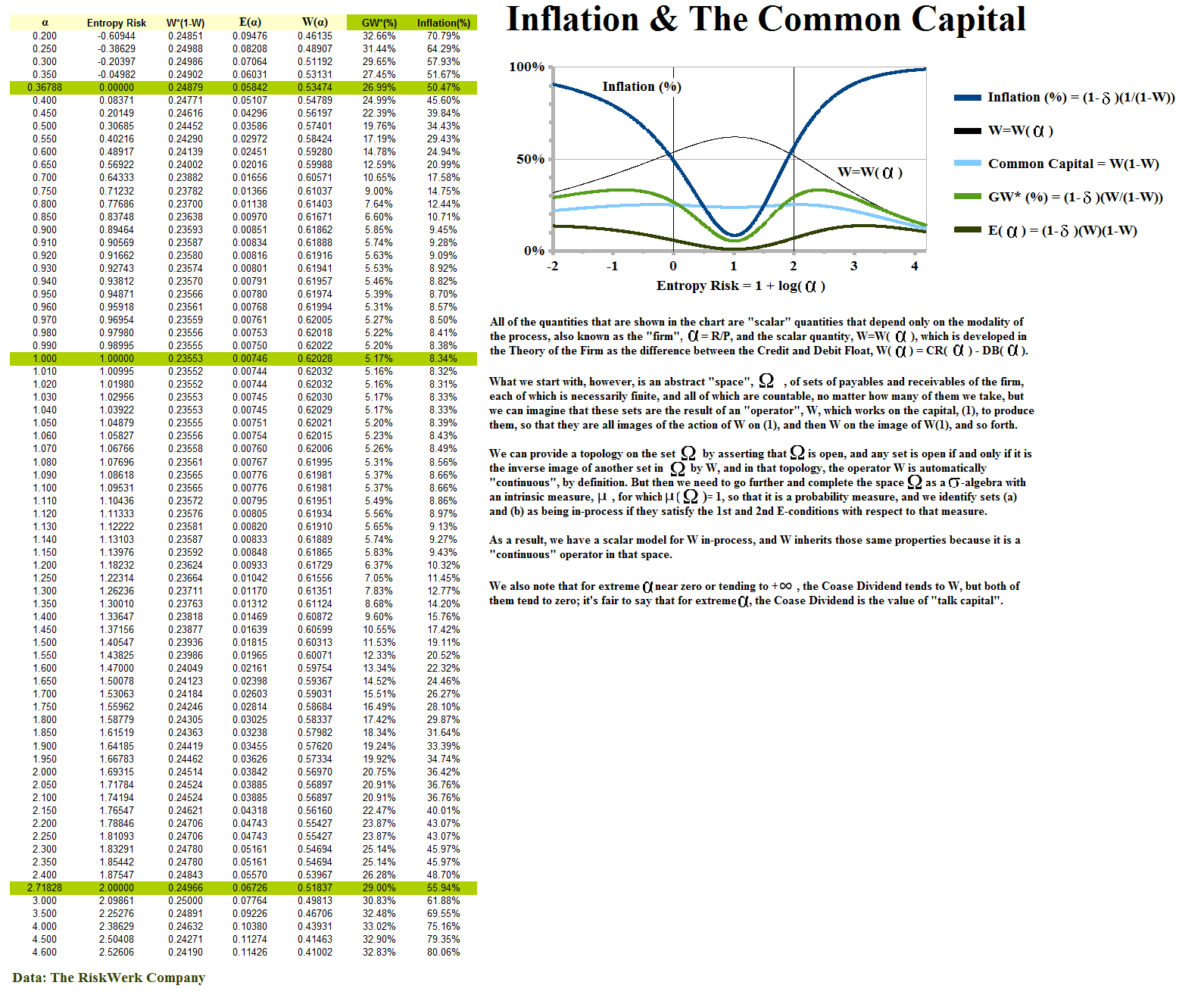
Figure 3: Inflation & The Common Capital
The least value of the “inflation” is 8.3% and it occurs at a modality of α=1, and is very close to that in a neighborhood of α≈1, including the largest “Profit Box” which occurs at about α≈1.10; however, “exact” is not an option because the actual numbers are “irrational” and not available in a closed-form, although the theory suggests that the minimum inflation occurs exactly at α=1, but then, it’s only approximately 8.3%; please see Figure 3 on the right for a table of values for the “inflation” and GW* in-process.
The “uptake rate”, in years, is then the time that we require in order for the “vapor”, which we have called the “inflation” and which depends on the modality of the process, to materialize as a (1), and because we are using the log-forms, that “time” is the ratio of the inflation calculated for that modality divided by the slope of the line, log(GDP*), for example, or log(Trade*) for the Trade Modality.
Inflation(%)/Δlog(GDP*)
If the uptake rate, in years, is increasing, then the rate of growth is slowing, and we are in a deflationary economy; whereas if it’s decreasing, the rate of growth is increasing and we are in an inflationary economy which supports that growth, but doesn’t predicate it (or drive it); please see below for examples in the current real economies, and Exhibit 1 below for a detailed explanation of “The Barometer”.
We’ll also find that it is very hard, almost impossible, for an economy not to be in a deflationary mode, if it makes economic sense; and it is also rare that the GDP* is growing without also an increase in the trade, Trade*.
The One World Food Bank
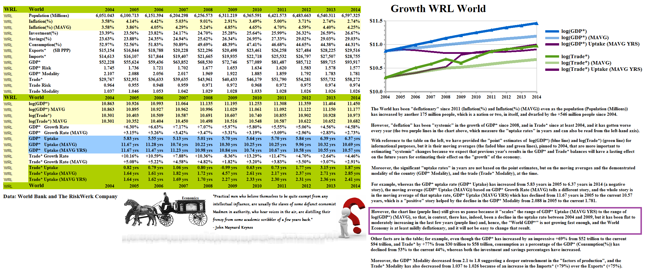
Figure 4: Practical Men
The One World Food Bank is, obviously, controversial, but unlike the “practical men” of Mr. Keynes’s famous dictum, we are not slaves to any economist, nor to the “mad men” (if there are any because there are none who claim to be) that govern us.
In that regard, however, there are only three types of government that we might have to deal with; there are the “Tories” or “Republicans” who want the price of an income to be high and, therefore, want to maintain a deflationary environment; and there are the “Liberals” or “Democrats” who want the price of an income to be low, or affordable, and therefore, prefer an inflationary environment sustained by growth; and there are the “totalitarians” who want everything to be “free” (socialists) or everything to be theirs (fascists, no matter what book they’re reading from), and, in practice, there’s no difference between them; please see Figure 4 on the right for some definitions and even more vital data.
In order for an economy to be growing, the “uptake rate”, in years, for the GDP* needs to be declining or, at least, not increasing, and the opposite is usually preferred for the trade in Trade*; and unlike the assumption of a natural inflation rate of +8.3% corresponding to a trade modality of about 1.1 (as in Figure 1 above), we need to consider both the Country Risk and the Trade Risk according to whatever modality they demonstrate at the time.
To get those rates, we calculate the point estimates based on the annual data (such as log(GDP*)); then their moving average pinned to the start year, 2004 (log(GDP*) (MAVG)), in order to remove short-term volatility; and then the point uptake rates, in years, that derive from the then current modality (such as GDP* Modality, which is calculated for each year, and remains a point estimate) of the then current moving average of the log-forms (log(GDP*) (MAVG)) to obtain log(GDP*) (MAVG YRS) and log(Trade*) (MAVG YRS), which are the “systemic” uptake rates in each year.

A “balanced budget” they say. What does it do?
Please see Exhibit 1 below for a detailed example applied to Canada, which has been “robustly deflationary” for the last several years, despite government “uncertainty” and “perplexion” and a “balanced budget”, from all of which it might be relieved in the upcoming election, but it is far from alone in that category; please see Exhibit 2 below.
Exhibit 1: CAN Canada – The New Fundamentals and a Balanced Budget
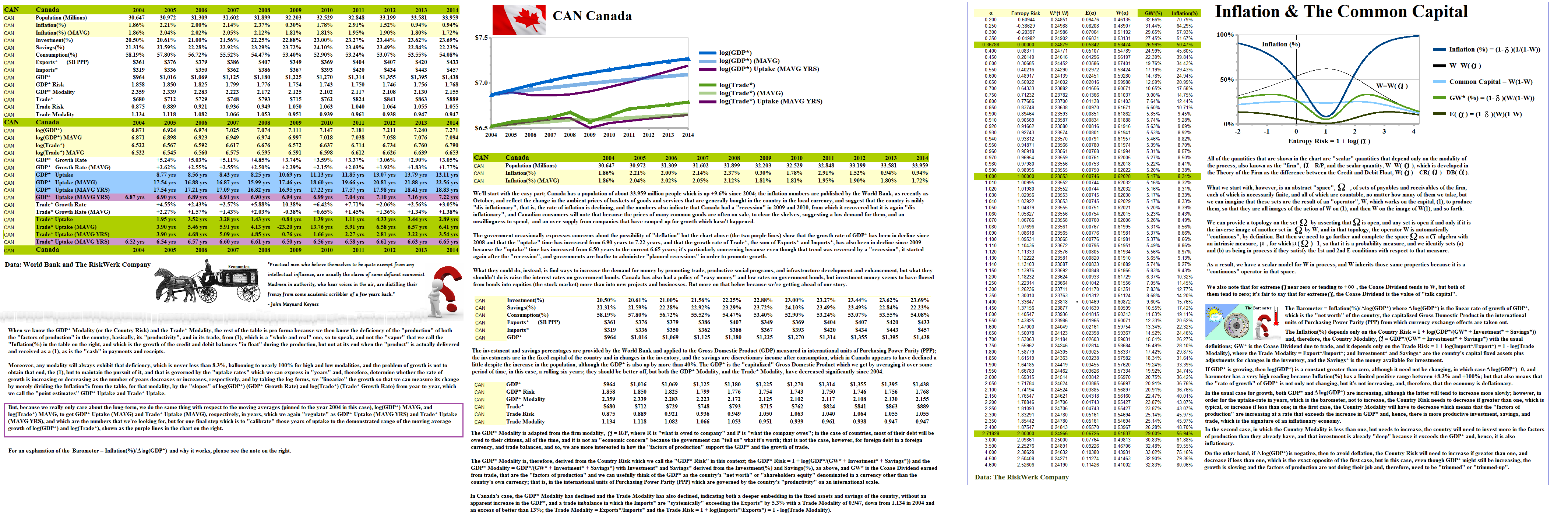
Figure 1.1: Growth CAN Canada – Data
Every country, and we have 185 of them in our database with data from the World Bank and the International Monetary Fund (IMF), has a chart and data that are similar to that of the WRL World and CAN Canada, above, and we’ve put together more than a dozen of them from the north, east, south and west, in Exhibit 2 below; please click on them to make them larger, and again if required.
Exhibit 2: The One World Food Bank
|
Figure 2.1: USA United States RUS Russia |
Figure 2.2: CHN China JPN Japan |
Figure 2.3: CAN Canada GBR United Kingdom |
|
Figure 2.4: DEU Germany FRA France |
Figure 2.5: FIN Finland SWE Sweden |
Figure 2.6: UKR Ukraine SYR Syria |
|
Figure 2.7: ISR Israel ITA Italy |
Figure 2.8: ESP Spain PRT Portugal |
Figure 2.9: GRC Greece KOR Korea |
|
Figure 2.10: MEX Mexico BRA Brazil |
Figure 2.11: ARG Argentina VEN Venezuela |
Figure 2.12: IND India IDN Indonesia |
|
Figure 2.13: AUS Australia ZAF South Africa |
Figure 2.14: EGY Egypt NGA Nigeria |
Figure 2.15: IRN Islamic Republic of Iran SAU Saudi Arabia |
The Food Locker – Productivity & Trade
We’ve avoided making comments on the charts because each situation is unique; all that we can say, in general, is that a dip in the Trade* uptake-rate (which is inflationary because we should expect that the price of an income and trade-related assets that produce it, will go down) is likely to result in a recession, particularly if the government depends on trade for an income and can’t boost the interest rates on its debt, for more debt; beyond that, a country will need to know what it is about its investments, savings, consumption, and trade, that are obstacles to growth.
We noted above that it is very hard for an economy not to be deflationary, and we can measure the challenge, or depth, of deflation by the “barometer”, Inflation(%)/Δlog(GDP*) and Inflation(%)/Δlog(Trade*), of which the latter is the most susceptible to change – if it’s increasing it’s likely that there is a robust trade development, whereas if it’s decreasing, or likely to decrease, there is, or will be, a “trade recession” which will also affect the growth of GDP*.
Inflation(%)/Δlog(GDP*)
Inflation(%)/Δlog(Trade*)
For example, the ratio, Inflation(%)/Δlog(GDP*), is intrinsically unstable because the numerator, Inflation(%), has a well-defined positive range between 8.3% and 100%, whereas the denominator, Δlog(GDP*), could be zero, or close to zero, indicating a very slow, or constant, economic growth, which has to change sooner or later, and therefore, there will be a change in its rate, Δlog(GDP*), which is either positive or negative; to effectively speed it up, the country would need to either increase the Country Risk if it’s low, or decrease the Country Risk if it’s high, and it can only do that by increasing the productivity of its economy, and it helps if it can also increase the productivity of its trade, so that Trade Risk = 1 – log(Trade Modality), is closer to one; please see Exhibit 1 above for further explanations.
Figure 5: LBY Libya SSD South Sudan
Only three countries have had an actual decline in the GDP* since 2009; Greece (please see Figure 2.9 above), Libya, and the South Sudan (please see Figure 5 on the right); of these, the “barometer” is still pointing up for Greece meaning that the uptake-times are increasing, and not only is the rate of growth of GDP* negative, it is increasingly negative, and the modest improvements in the Trade Risk have not been able to reverse that decline.
The issue of “growth” is not whether there will be “more” – there will always be more – but will it arrive in time?
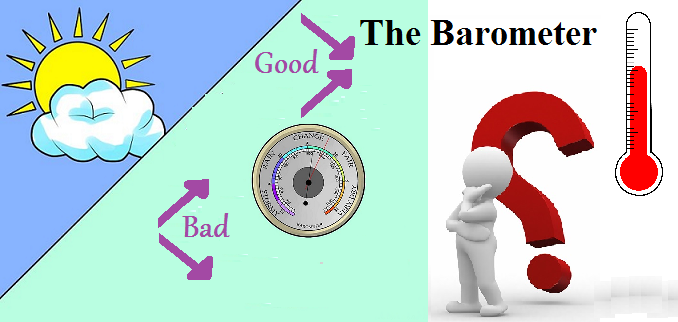
If we think of the barometer settings as “arrows” then GDP*(down) and Trade*(up) is the best because it indicates a high productivity in both the production of GDP* and the Trade*; GDP*(up) and Trade*(up) might still work if the trade is strong enough to sustain a faltering economy; GDP*(up) and Trade*(down) is the worst because it demonstrates both a faltering economy and a diminishing benefit from trade; however, GDP*(down) and Trade*(down) might still work if the strong economy is able to offset the diminishing benefit of the trade; hence, (up)(up) and (down)(down) might be OK; (up)(down) is not OK, but (down)(up) is the best.
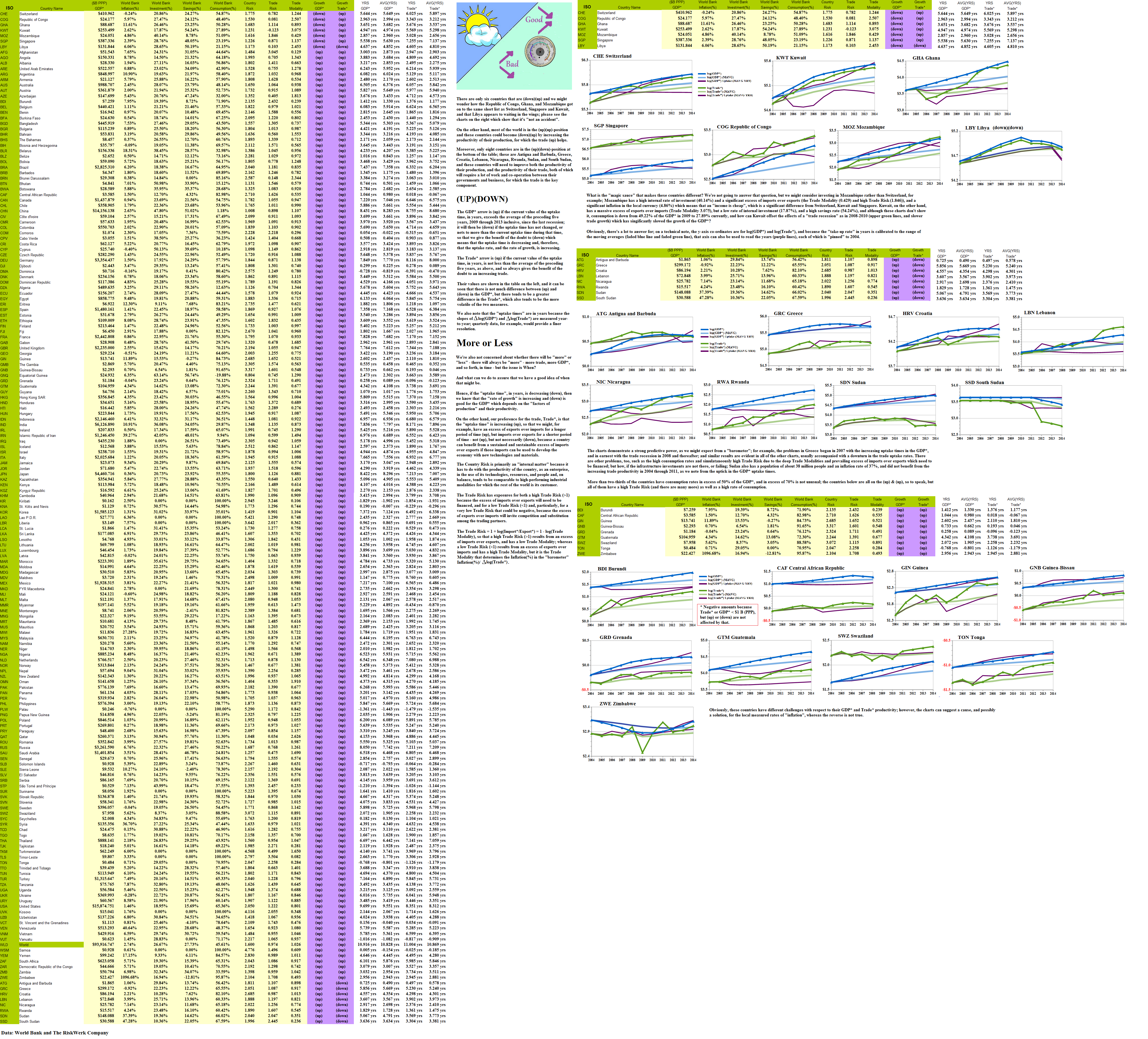
Figure 6: The Barometer
Moreover, a country cannot maintain a constant rate of growth indefinitely; that is, Δlog(GDP*)=0, or Δlog(Trade*)=0, or close to it, although it is possible that a country could sink to the bottom and stay there pending a war or revolution, notwithstanding what the countries at the “top” might do in order to maintain their position; but because change is required, we need to avoid a transition from (down)(up) to (up)(down), which is a “disaster”, by “buffering” change as (down)(up) to (down)(down), or (up)(up), before returning to (down)(up), and avoiding (up)(down) altogether; please see Figure 6 on the right for some examples – most of the world is currently (up)(up) and these countries need to work at getting some (down)(up), but that’s a local problem and best that they know that they have it.
The “benefit” of the trade depends on the Trade Risk = 1 + log(Import*/Export*) = 1 – log(Trade Modality); if the Trade Risk is high (>1), then the imports are exceeding the exports and the benefit could be in sustaining the people with imported goods, or in developing the country infrastructure with new technologies or materials; if the Trade Risk is low (<1), then the exports exceed the imports and the risk is in inviting competition and substitution for the exported goods and services.
Our preference for the trade is that it be (up) and, therefore, that the uptake-times are longer so that the benefit of the trade, which is hard-won in the development of the trading connections, can work its way into the economy.
Because of the importance of trade, we’re motivated to have a look at some of the smaller Euro-area economies that are emerging economies and highly dependent on trade, in many cases exceeding the GDP*; please see Exhibit 3 below.
Exhibit 3: Euro-area Developing Countries
|
Figure 3.1: EST Estonia LVA Latvia |
Figure 3.2: LTU Lithuania POL Poland |
Figure 3.3: HRV Croatia SRB Serbia |
|
Figure 3.4: BGR Bulgaria ROU Romania |
Figure 3.5: MDA Moldova AUT Austria |
Figure 3.6: HUN Hungary BLR Belarus |
For more information on real “risk management” in modern times and additional references to the theory and how to read the charts and tables, please see our Post, The RiskWerk Company Glossary and “(P&I) Dividend Risk and Dividend Yield“, and our recent Posts “(P&I) The Profit Box” and “(P&I) The Process – In The Beginning“; and we’ve also profiled hundreds of companies in these Posts and the Search Box (upper right) might help you to find what you’re looking for, such as “(B)(N) TLM Talisman Energy Incorporated” or “(B)(N) ATHN AthenaHealth Incorporated” or “(B)(N) PETM PetSmart Incorporated“, to name just a few.
And for more applications of these concepts please see our Posts which rely on the Theory of the Firm developed by the author (Goetze 2006) which calibrates The Process to the units of the balance sheet and demonstrates the price of risk as the solution to a Nash Equilibrium between “risk-seeking” and “risk-averse” investors within the demonstrated societal norms of risk aversion and bargaining practice. And for more on The Process, please see our Posts The Food Chain and The Process End-Of-Process.
And for more on what risk averse investing has done for us this year, please see our recent Posts on “(P&I) The Easy (EC) Theory of the Capital Markets” or “(B)(N) The Easy (EC) Theory of the S&P 500“, and the past, The S&P TSX “Hangdog” Market or The Wall Street Put or specialty markets such as The Dow Transports & Utilities or (B)(N) The Woods Are Burning, or for the real class action, La Dolce Vita – Let’s Do Prada! and It’s For You, Dear on the smartphone business.
And for more stocks at high prices, The World’s Most Talked About Stocks or Earnings Don’t Matter – NASDAQ 100. And for more on what’s Working in America, Big Oil, Shopping in America or Banking in America, to name just a few.
Postscript
We are The RiskWerk Company and care not a jot for mutual funds, hedge funds, “alternative investments”, the “risk/reward equation” and every other unprovable artifact of investment lore. We have just one product
The Perpetual Bond™
Alpha-smart with 100% Capital Safety and 100% Liquidity
Guaranteed
With No Fees and No Loads on Capital
For more information on RiskWerk, please follow the Tags or Categories attached to this Letter or simply enter Search for additional references to any term that we have used. Related data may be obtained from us for free in a machine readable format by request to RiskWerk@gmail.com.
Disclaimer
Investing in the bond and stock markets has become a highly regulated and litigious industry but despite that, there remains only one effective rule and that is caveat emptor or “buyer beware”. Nothing that we say should be construed by any person as advice or a recommendation to buy, sell, hold or avoid the common stock or bonds of any public company at any time for any purpose. That is the law and we fully support and respect that law and regulation in every jurisdiction without exception and without qualification to the best of our knowledge and ability. We can only tell you what we do and why we do it or have done it and we know nothing at all about the future or the future of stock prices of any company nor why they are what they are, now. The author retains all copyrights to his works in this blog and on this website. The Perpetual Bond®™ is a registered trademark and patented technology of The RiskWerk Company and RiskWerk Limited (“Company”) . The Canada Pension Bond®™ and The Medina Bond®™ are registered trademarks or trademarks of the Company as are the words and phrases “Alpha-smart”, “100% Capital Safety”, “100% Liquidity”, ”price of risk”, “risk price”, and the symbols “(B)”, “(N)” and N*.
