(P&I) The Process – The WalMart Company B Story
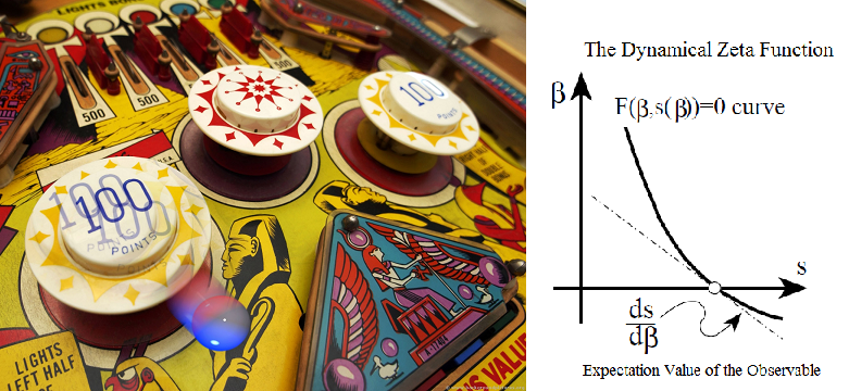
Courtesy: Chaos Classical and Quantum, Cvitanovi’c et al.
Essay. The System Dynamics of The Process is similar to a game of “pinball” with three throbbing orbs that change in size while we’re playing; please see Figure 1.1 below for an example.
However, unlike pinball, The Process is regulated by “risk” that is defined by “the societal standards of risk aversion and bargaining practice” (please see The Theory of the Firm) and which prevents the collisions from occurring with the same unerring finality of the mathematical pinball machine, which has no “friction” and no solution, even if the orbs aren’t “throbbing”.
However, something can be done if the orbs are “throbbing” (or not) in a regular way, such as in a heartbeat with its two sets of chambers and a muscle; or the helium atom, He, with a dense nucleus and two electrons; or the earth-moon-sun system, all of which appear to be somewhat “stable” absent a random event, and all of which are examples of The Process in the right co-ordinates with probabilities a=p((a)) and b=p((b)) that can be shown to require the 1st and 2nd E-conditions, which are always required if there is counting and entropy is conserved.

Figure 1: The 1st Real Dollar
We’ve also discovered that the real “worth” of the dollar is decided in the cauldron of the subsistence economy by the process of exchange at the Company D modality, where governments also dwell, and new companies form, and from which escape is only made possible by “random events”, which are just sets of measure zero in the larger scheme of things.
And we’ve crafted investment portfolios in “The Easy (EC) Theory” of the markets, which meet our criteria for investments (and not gambles) – safe, liquid, and hopeful – and don’t depend on systemic random factors such as “volatility” (which is just noise), but could still depend on the willingness, and ability, of investors to invest, which factors we don’t know how to forecast, but which we do know how to control for, or “dampen”, by considering the “risk” of such investments with respect to our criteria of safe, liquid, and hopeful; please see Exhibit 3 below.
Whereas the Company E (α=1) and C (α>1) modalities always have access to lots of “cash” (receivables) to effect the end-of-process, and Company D (α=1/e) always needs some “cash” (beg, borrow, or steal) to effect the end-of-process (and we know how much), Company B with modality, 1/e < α < 1, is more “industrial” and has negotiable and navigable sets of receivables (b) and payables (a) throughout its process; please see Exhibit 1 below, and our Post “(P&I) The Process – End-Of-Process (E,C,D)” for more information.
Exhibit 1: Company B at the WalMart Modality α=0.74
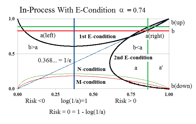
Figure 1.1: In-Process Company B α=0.74
All the elements that we’ll need to talk about are in this chart, and in order to effect the end-of-process at a=b=1, we’ll need to look more closely at the lower right corner where (a) is “mapped” to a sequence of a’→1, and (b) to a corresponding sequence of b(down)→0.
And, in the usual notation, a=p((a)) and b=p((b)) where (a) and (b), and so forth, are sets in the σ-algebra defined by the process and a=p((a)) is the measure, or probability, of the set (a).
Since we are in-process with modality α=0.74, Company B has established relationships with its trading connections, which include, for example, its suppliers, employees, and customers, and for which sets of payables, (a), that are drawn on Company B, are in-process with sets of receivables, (b), that are drawn in the trading connections, and they are related by the 1st and 2nd E-conditions, a×log(a) = α×log(b), and b×log(b) = α×log(a), respectively, which are a necessary consequence of merely counting and matching in the context of a “Conservation Law”, which is the “Balance Sheet” in this context; please see The Process for more details.
With reference to Figure 1.1 above, if a=a(left)=p((a(left))) is a set of payables of Company B that is in-process, then there is a set of receivables b=p((b)) for which the 1st E-condition obtains; and also another set (a) = (a(right)) and another set (b) = (b(a(right))) for which p((a(left)))<p((a(right))) and b=p((b(a(left)))=p((a(right))), but which has “advanced” the process from a(left) to a(right) which is much closer to the end-of-process at a=b=1; please see Exhibit 1, above, for the “picture” of how this is done.
The Cantor Set
We will often short-hand the notation, but it’s important to note that we don’t expect that any of these sets are the same, only that they have the appropriate measures that satisfy the 1st and 2nd E-conditions, as is required by “in-process”.
Moreover, any of these sets may differ by sets of measure zero, which would include all “countable” sets of payables and receivables, and so render the accountant unable to help us; in fact, sets such as (a) and (b) that satisfy the 1st and 2nd E-conditions, always have the power of the continuum because, for example, by the 1st E-condition, a = α×log(b)/log(a), and the factor, log(b)/log(a), is the fractal or Hausdorff dimension of the set (b) as a “covering set” for (a) – which, in fact, is what receivables do – they “cover” payables; please see our Post “(P&I) The Process – Commensurability” for more information.
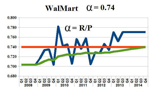
Figure 2: WalMart Modality α=0.74
However, it’s easy to calculate the modality for a real company, such as Wal-Mart Stores Incorporated, from their quarterly or annual balance sheets; please see Figure 2 on the left which shows the actual R/P (blue) as calculated from the quarterly balance sheets, and estimates of the same from these data, the average (red) and the moving average (green).
The modality is, α=R/P, where (P) are the “total liabilities” and includes everything above the “shareholders equity” and, so, it includes all the debt (short- and long-term), minority interest, if any, and preferred shares; we usually say that (P) is “what the company owes” and that (R) is “what is owed to the company” in an “economic sense”; that is, (R) is the total assets plus the “accumulated depreciation” less “what it owns”, which are the “inventories” and net plant and equipment, or fixed assets.
Please see The Theory of the Firm for more details, but we note that “accumulated depreciation” is a “cipher” and is related to what the company needs to maintain in order to do its “business”, for which the fixed assets and “inventories” should also be considered as “ciphers”.

The Banking Crisis
For example, we might consider “stocks on the shelf or for trade” as a part of the “inventory” of banks that do a lot of investment business, or merchant banking, and, in those cases, it might change a Company C modality (α>1) which is typical for a deposit-taking and loan-making bank, to a Company B modality which puts an entirely different demand on the bank’s payables and receivables, as we have seen in the “banking crisis” of 2007 and 2008; please see below.
In general, however, the modality is hard to change and any modality in a Company B, 1/e<α<1, demonstrates similar properties, with extremes in those properties near α=1 (Company E) and α=1/e (Company D), in which the Company B “behaviour” becomes “exaggerated” in a way that is similar to what we observe, for example, when ordinary water is chilled to the freezing point, or heated to the boiling point.
The modality is a “state measurement” and we have shown that its value is the “entropy” of the process as Ω(b) = -∫ b(a)×log(b(a))da = -∫α×log(a)da = -α×[a×log(a) – a] = α on [0,1]; please see our Post “(P&I) The Process – System Dynamics” for more information.
The Fundamentals of Company B
The “fundamentals” for WalMart, and companies in a similar business, which is the business of “converting inventory” to “earnings”, are shown in Exhibit 2 below.
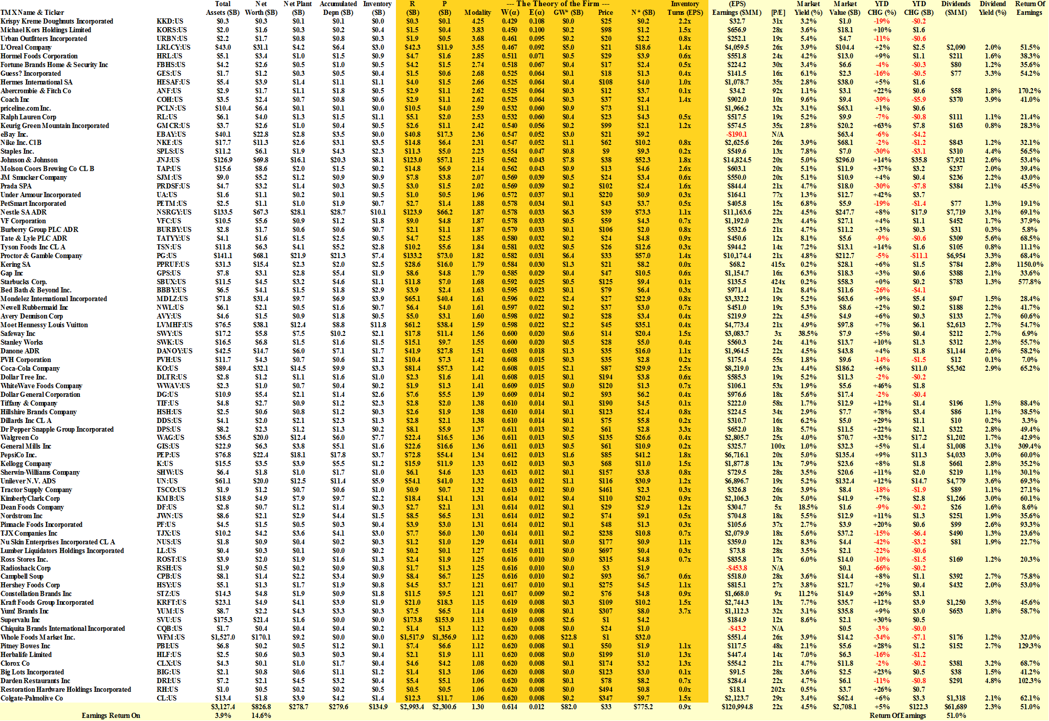
Exhibit 2: Wal-Mart Stores Incorporated – Fundamentals
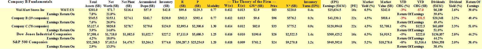
Figure 2.1 Company B Fundamentals – Summary
The details, and their meaning, are developed in The Theory of the Firm; however, it’s helpful to have some examples of the Company B modality in front of us, and it’s also a result of the theory, which is provable in economics and mathematics, that there are only a few things – none of which are in common use, but for which there are a lot of unprovable substitutes – that are pertinent to the financial analysis of a company and the company’s stock prices, which are not theoretically correlated, but are correlated through an observable that we call the price of risk; please click on the chart (and again) to make it larger if required.
The accounting entries and the calculation of (R) and (P) are shown on the left-hand side of the table; E(α) and W(α) are defined in The Theory of the Firm, but their values are not meaningful without their consequences, which are GW* and N*.
GW* is the “balance sheet worth of the trading connections” in the sense of Coase (the economist, Ronald H. Coase, 1910-2013) which we call the “Coase Dividend” and it is in the same units as the balance sheet, which could be in any currency; it is a “capitalization” of the company’s “work” in developing the trading connections, for which it exists, and who are its suppliers, customers, employees, creditors, shareholders, and so forth, and which “activity” results in, and is the cause of, the company’s “payables” (what it owes) and “receivables” (what is owed to it).
The market value of the company posits a “price” for the Coase Dividend, so that, in the case of WalMart, investors are willing to pay $83 for $1 of the Coase Dividend, which is about three times what investors are willing to pay for the Coase Dividend of all the companies in the S&P 500 ($24) or the Dow Jones Industrials ($26); please see Figure 2.1 above.
On the other hand, there are nineteen companies that have a “problem” (or “business”) similar to that of WalMart, all of which have a Company B modality, and the aggregate value of the Coase Dividend is $96 for $1 of the Coase Dividend; and there is a much larger group of similar companies (78 companies) that are Company C, with a modality α>1, for which investors are willing to pay an aggregate amount of only $33 for $1 of the Coase Dividend; please click on the links “Company B Fundamentals” and “Company C Fundamentals” for more details.
However, the Coase Dividend for all of these companies measures exactly the same thing – it is the balance sheet worth of the trading connections – and $1 of it in one company is the same as $1 of it in another company; investors, however, are “pricing the future” – rightly or wrongly – and, as another example, pharmaceutical companies that are developing new drugs and treatments will have a “Coase Dividend” that trades at well over $100 or more, until their hopes are confirmed or denied.
We never gaze into the future, but we can calculate what it will be worth based on what we know now, and that value is N* which is the result of “compounding the working of the Coase Dividend” from now until then, although “then” doesn’t have any “time” attached to it; it is a “state” measurement.
For example, the current net worth, (N), of the WalMart Company is $72 billion, and the value of (N*) is $220 billion, so that, over time, just by doing what it does, day-in and day-out, Monday through Friday (and Saturday and Sunday too), we expect that the net worth of the WalMart Stores will be more than three times (3.1× = $220/$72) what it is today, whereas the aggregate of companies similar to WalMart in Company B is (3.8× = $577/$153), and in Company C ( 0.94× = $775/$827), and those numbers reflect only differences in how the companies go about their “business” which is the “business of creating payables and receivables” and, hopefully, “earnings from inventory”, from what they have, regardless of what they actually make or do.

What? And so what?
As a result, we are generally uninterested in the actual or forecast “earnings” of a company, although we calculate the “capitalization rate” of earnings from inventory with the ratio “Inventory Turns (EPS)” which is 0.4× ($15.6 billion/$42.8 billion) for WalMart; please see Exhibit 2 above.
The logic is that if “E” is the earnings (which is a “balance sheet” number at this point and will be added to the net worth net of dividends) and “I” is the inventory, then E = I×exp(log(E/I)) = I× exp(r) with r= log 0.4 = -0.92, which means that the “earnings” are trading at a discount to the inventory and, therefore, it’s a “low margin” business, but still a higher margin than the rest of the similar companies which are trading at r=log(0.3)=-1.2, and a 30% decrease in the rate of “earnings accumulation” from “inventory”; Mead Johnston Nutrition Company, Phillip Morris International, and Lorillard, all show a much higher “added value” to their inventory; for more details, please click on the link “Company B Fundamentals“.
Exhibit 3: (B)(N) Wal-Mart Stores Incorporated – Risk Price Chart

Figure 3.1: (B)(N) Wal-Mart Stores Incorporated – Risk Price Chart
The Theory of Firm calculates (N*) in abstract units and shows how to project, or “illuminate”, those values in the balance sheet; it also shows that the “price of risk” is an indifference price which resolves a Nash Equilibrium between “risk seeking” and “risk averse” investors which is, then, the “fair price” for a stock with a built-in bias for returns above the price of money (inflation).
However, stocks don’t trade “fairly” for long and a stock that is trading at or above its price of risk, is “undervalued” because there is an excess of demand over supply for the stock at those prices, however “high” they might be; and a stock that is trading below the price of risk is “overvalued” because there is an excess of supply over demand for the stock at those prices, however “low” they might be, and they could be zero, or anything else, due to the demonstrated investor “uncertainty” about their “worth”, for one stock, or many, all at the same time, for some “reason” yet to be discovered.

Volatile, but they can be frozen, or vaporized.
With respect to Figure 3.1 above, the stock of WalMart is “undervalued” and an attentive stop/loss policy can lock in price gains which, in this case, are equivalent to 9% per year despite the “volatility” which is (provably) “irrelevant” to the fair pricing of stocks on a portfolio basis; moreover, if the stock is still trading above the price of risk, we can buy it back at a lower price which, generally, adds to the returns above cash and dividends.
Company B End-Of-Process & Process Risk
It’s helpful to think of the Company B, in-process, as the “producer”, and its trading connections as the “customer”, in which Company B could be anything from one company, to a market, or an entire economy; please see Exhibit 4 below.
In principle, the process can be thought of as beginning in the upper left-hand corner with a=0 and b=1, and ending in the upper right-hand corner with a=1 and b=1 (again); all that means is that the payables, (a), at the “beginning of process” are at most countable and have zero measure, whereas the “rest of the world”, the trading connections (b), has everything else, and that’s a scenario that we looked at in explaining the “1st Real Dollar“.
Moreover, we can also show that there is never an end-of-process at a=1 and b=1, but that we are always tending towards the end-of-process when we are in-process, and that there are the means to do it in-process.
If (a) and (b) are sets of payables and receivables in-process, then we can call, Risk(a) = 1 – log(1/a) = 1 + log(a), the “producer risk”, and Risk(b) = 1 – log(1/b) = 1 + log(b), the “customer risk” for the sets (a) and (b) that are in-process, where we note, as above, that log(1/a) is the “capitalization rate” of (1) by (a); that is, if r=log(1/a), then 1 = a×exp(log(1/a)) = a×exp(r).
We also note than when (a) or (b) have measure close to zero, or a<1/e, for example, then the risk is negative or even vastly negative, meaning no risk to the bearer, and that zero risk occurs at a=b=1/e, and that “total risk” (100%) occurs at a=b=1, which signifies “ownership” as a “cash equivalent” outside the domain of production.
Exhibit 4: The End-of-Process In-Process Company B (α=0.74)
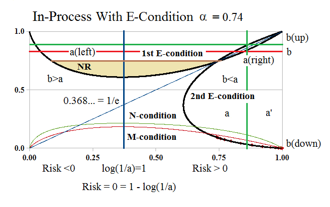 Figure 4.1: In-Process Company B α=0.74 |
 Figure 4.2: In-Process Company B At End-Of-Process |
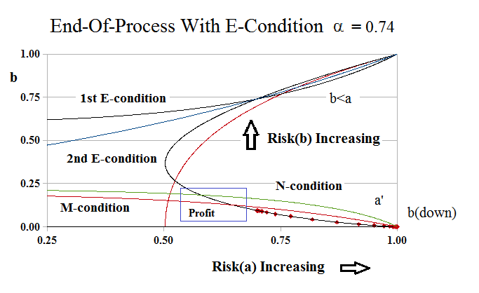 Figure 4.3: Profit & Risk At End-Of-Process |
With reference to Figure 4.1 above, we noted that Company B, in-process, never starts at a(right)=0 and b=1, but at some point a(left)>0 and b<1, where, as usual, we are talking about the sets of payables and receivables, (a(left)) and ((b)), which are required to exist in-process.
But where it starts is determined by the “profit motive” which is executed between the “producer” (a) and the “customer” (b) in the “blue box” in the lower-right corner of Figure 4.3, which is close to the end-of-process at a=b=1, and where the co-ordinate sets are (b) on the vertical axis, and Risk(a) = 1 – log(1/a) = 1 + log(a) on the horizontal axis; please click on the charts to make them larger if required.
The “line of dots” on the 2nd E-condition, b×log(b)=α×log(a), in each of the charts shows the progress of production from a(left) to a(right) to a’ and b(down), and the progress will always be similar to that as long as b=b(a(left))>α, which occurs at the intersection of 1st and 2nd E-conditions at α=0.74, and that number can be readily calculated as the solution a=a(left) where a×log(a) = α×log(α) (by a Newton-Raphson method) and a(right)=α; please see Figure 4.1 above.
We’ll call the number “NR” so that if a(left)<NR, then b=b(a(left))>α, and if NR≤a(left)≤α, then b=b(a(left))≤α, and for such a(left) there appear to be no implementing sets (b) and b(up) that will allow the process to “advance” from a(left) to a(right) and a’; and we’ll also call the set of all such (a) and (b), NR, which is the shaded “basin” in Figure 4.1 above.
To help the “producer”, we know that for all such a∈NR, there are in-process sets of receivables such that b>a, and that the “risk” to the producer is negative, Risk(a)<0, as long as a<1/e, and positive thereafter; moreover, the “risk” to the “customer” is also negative as long as Risk(a) = 1 + log(a) < 1-1/(α×e) =0.502866… in this case; please see Figure 4.3 and Figure 4.4 below for an update of this “NR-problem”.
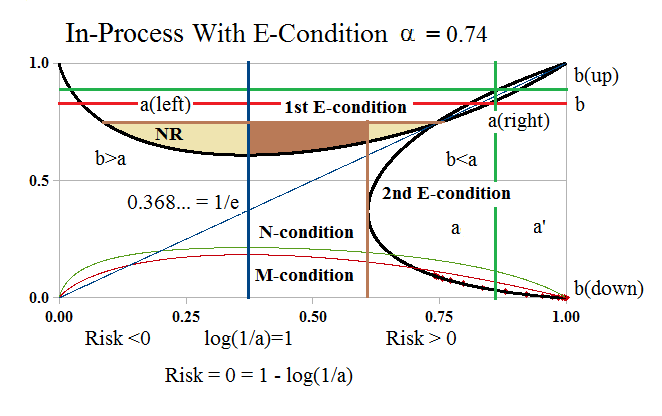
Figure 4.4: The NR-problem
The “NR-problem” exists for all the Company B modalities, 1/e<α<1, because it is defined precisely by boundaries that depend only the modality and which don’t disappear until α≤1/e (Company A and D) or α≥1 (Company E and C).
Moreover, the “basin” is long and shallow for α near α=1, which is the Company E modality, and disappears to a “point” at α=1/e, which is the Company D modality.
The producer could forge-on through this “basin” by acquiring more “payables”, that is, labour, materials, et cetera, because there is a set of receivables, (b), for every occasion in the NR-basin, and b>a during all of it; in practice, the producer might get receipts, or credit, or factor their receivables, to meet the demands of the situation; and there is no risk to the producer until they forge-on past a=1/e, nor is there any risk to the customer until the producer has forged-on past (a) where Risk(a)>1-1/(α×e) =0.502866… (as above), at which point both the producer and the customer are “at risk”.
And the risk is that the producer might not be able to produce the “product”, which is (1), and the customer might, therefore, not be able to receive it, or, if it is produced, might not be able to buy it, despite all of the hardship. The solution is to never get into the basin, but if we are in the basin, then we need a “random event”, an event of measure zero, to either cancel the payables and bring us back to a(left)<NR, or raise both the payables and the receivables past a=b=α.
Figure 4.5: Profit & Risk At End-Of-Process
In order to avoid the problem in the “future”, we need to look more closely at what needs to be done at the end-of-process; please Figure 4.5 on the left which is the same as Figure 4.3 above.
If we are past the “basin”, then the line of “dots” on the 2nd E-condition shows the production path as (a) is increasing towards (1), and (b) is also increasing towards (1), but (b)=(b(down)) is decreasing towards zero, and that progression, or “state of affairs”, is a certainty towards a certain end, a=b=1, which it never attains.
It’s also noteworthy that all of these measurements are “state measurements” and that “time” does not exist as long the company is in-process and therefore preserves the entropy, which is the modality, α, and the meaning of “in-process”.
Moreover, any decisions that the producer or customer makes are “random events” of measure zero, and may be “out-of-process”, in practice, although not necessarily so.
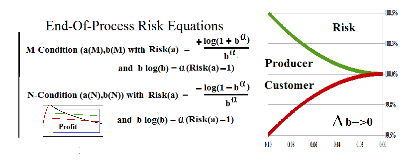
Figure 4.6: In-Process Company B At End-Of-Process Risk Equations
The “blue box” that is shown in Figure 4.5 above, is actually too large, and it’s essential contents are defined by the “End-Of Process Risk Equations” (please see Figure 4.6 on the left) which we refer to as the “blue box”, and that is the one that we mean, with Risk(a(N))≤Risk(a)≤Risk(a(M)), in the “risk co-ordinates”, and b(N)≥b≥b(M) in the usual, linear, co-ordinates.
The company, then, can “cycle” in either of two modes: the “top mode” between a(left) and a(right) towards the end of production (which it never actually obtains but is always moving towards); and the “basin mode”, in all of (NR), for which the essential “blue box” defined by the end-of-process risk equations, is entirely contained in the “thin edge of the wedge” near a=b=α, on the right-hand side of (NR); and the difference between one “cycle”, or the other, is a “random event”.
However, we will show below that although the process can spin in the top-mode, so to speak, it prefers the “basin”, and absent a “random event” either for or against, it will “likely” go there, and that is where we will find it.
We also note that the “Risk Equations” can’t be solved using the usual methods because the limit, Δb→0 (please see Figure 4.6 above), needs to be taken “in-process” and the co-ordinates, (a,b), need to satisfy the second E-condition, b×log(b) = α×log(a) = α×(Risk(a) -1), in order to effect the limit in a way in which it might actually be realized; however, please see below (Entropy et al) for more information on the solution.
And, there’s a lot at stake – between ±50 basis points and ±2,000 basis points (±20%), or more, much more, depending on the modality; please see Exhibit 5 below.
Exhibit 5: The Real Risk at the End-Of-Process – How much risk would you like?
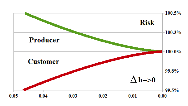 Figure 5.1: Risk α = 1.5 Company C (α>1.0) |
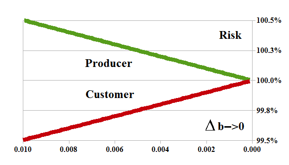 Figure 5.2: Risk α = 1.0 Company E (α=1.0) |
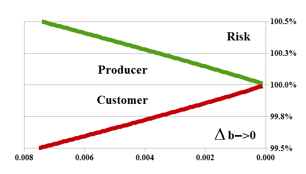 Figure 5.3: Risk α = 0.94 Company B (1/e<α<1) High Entropy |
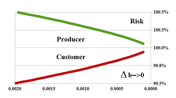 Figure 5.4: Risk α = 0.74 Company B (1/e<α<1) Normal Entropy |
 Figure 5.5: Risk α = 0.44 Company B (1/e<α<1) Low Entropy |
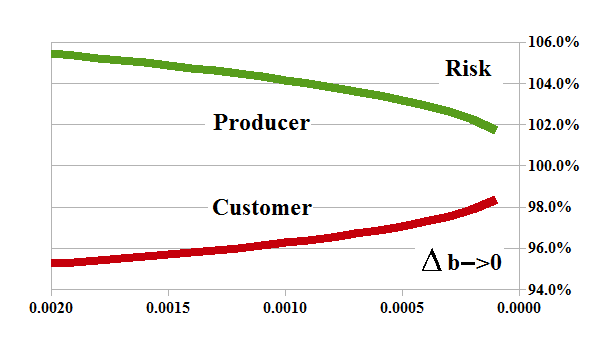 Figure 5.6: Risk α = 1/e = 0.368… Company D (α=1/e) The Death Embrace |
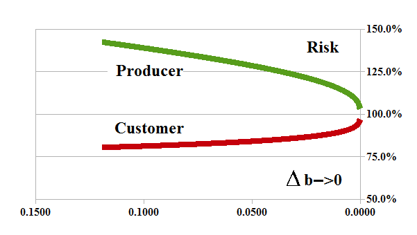 Figure 5.7: Risk α = 0.30 Company A (0<α<1/e) |
 Figure 5.8: Risk α = 0.20 Company A (0<α<1/e) |
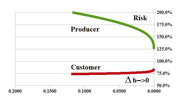 Figure 5.8: Risk α = 0.10617… ≈ γ/2e Company A (0<α<1/e) “Extreme Alpha” |
We can see from Exhibit 5, above, that the “Customer Risk” is only similar to the “Producer Risk” at high modalities, α≥1, Company E and Company C, and that the “risk profile” is convex up (please see Figure 4.6 for α=2), then more or less linear, and then convex down as the modality decreases; moreover, no matter how high the risk to the producer, the “Customer” is never on the hook for more than the “working capital loan”, 25% at risk (please see Figure 5.9 above), which is usually deemed as “unsecured”, net of the “inventory” and fixed assets (“what the company owns”), which are likely assigned to the “bond debt”; please see The Theory of the Firm for more details.

How much do you want?
We also note that “Producer Risk” levels of +30%, +50%, +100%, and so forth, above the “total risk” at 100%, assume that they want to stay in business, and will “deliver the product” (please see below for how that is done), and they have been “given” a generous opportunity to do so; failure to do so amounts to a “write-off”, “a gift”, or a “bankruptcy”, or, in the context of governments, a “currency devaluation” by declaration, hyperinflation, or default.
It is well-said that if we lend a person or company or government too much money, it becomes unclear who the “debtor” is, or will be, and that’s a situation that will affect many pension plans and endowment funds that do not or cannot “deliver”, and their “customers” who have financed these “payables”, in the years-to-come; please see our Post “The Pensionnaires” for more information.
Low, Normal, and High Entropy States in Company B
The charts below, in Exhibit 6, show the three states of Company B in which the modality is near Company D (α=1/e=0.368…) and “low entropy”; Company B at α=0.74 which we call “normal” in this context; and near Company E (α=1) and “high entropy”.
Exhibit 6: The End-of-Process In-Process Company B At Low, Normal, and High Entropy
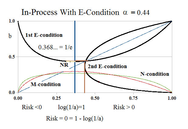 Figure 6.1: In-Process Company B α=0.44 Low Entropy |
Figure 6.3: In-Process Company B α=0.74 |
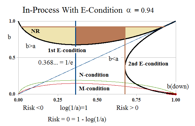 Figure 6.5: In-Process Company B α=0.94 High Entropy |
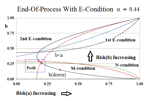 Figure 6.2: Profit & Risk At End-Of-Process Low Entropy |
Figure 6.4: Profit & Risk At End-Of-Process |
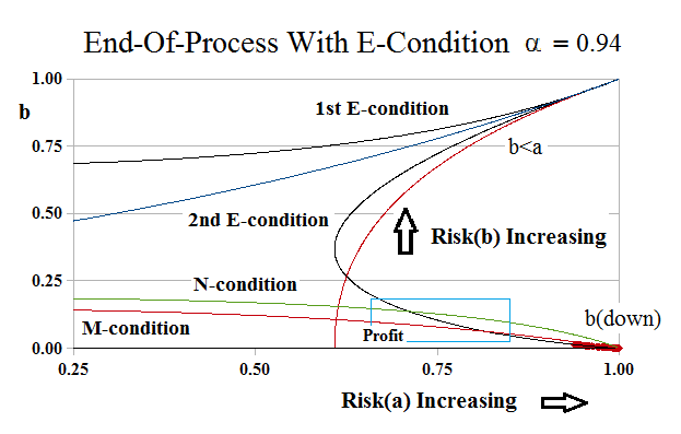 Figure 6.6: Profit & Risk At End-Of-Process High Entropy |
With reference to Exhibit 6, although there are many quantitative differences, the primary difference is qualitative. At low entropies (Figure 6.1 and 6.2 for α=0.44), the NR-region becomes very thin and eventually shrinks to a point in the “death embrace” at Company D with modality α=1/e=0.368… and, hence, the entropy is decreased; we also note that the M-condition takes effect at a lower risk, Risk(a), to the producer, than the N-condition, whereas the reverse is true at higher entropies.
On the other hand, at higher entropies (Figure 6.5 and 6.6 for α=0.94), the NR-region covers nearly the entire production space, and the right-hand side of it, at a=b=α, approaches the end-of-production at a=b=1; the exchange of “product”, which is payables (a) for the “delivery of product”, the “receivables” (b) which are the “price” for the delivery of product and the “receipt” of the product, is always done pro rata, that is, the producer has given (1) and the customer has paid (1) for it and they are the same (1), so that there appears to be no “profit” in the exchange.
However, as we noted above, “production” never begins at (0,1), nor does it ever end at (1,1), but rather, it begins at some a(left) and it ends at some a(right) which is governed by the “production” of receivables in the trading connections (the customer).
The 1st E-condition, a×log(a) = α×log(b), is the “production function” for the producer, but its reflection in the line a=b in the production space is the “production function” for the customer, and it is described by the 2nd E-condition, b×log(b) = α×log(a), but the co-ordinates (a,b) are the reflection of the co-ordinates (a,b) in the production space and, therefore, have a different meaning.
In the same way as the producer began production at a(left), the customer begins “production” at what we have called b(down) tending to b(up), and in that process, the customer has the same challenges and opportunities, in-process, as the producer, which we have summarized in Exhibit 6 above, because the production functions are the same but for a change in orientation; the producer produces payables and expects receivables at the end-of-process, and the customer produces receivables (which are their payables) and expects to receive the producer payables (its “product”, possibly encapsulated in something “tangible”) at the end-of-process, and the process is the same, in-process, in both cases and has the same “ending” at a=b=1.

Are You The One?
Hence, the M-condition, 1+log(a) = lim log(1+b^α)/b^α as b=b(down)→0, is not about “b→0” in the customer space, but about b^α = a^a→1 and a→0 at the end-of-production when the creation of additional payables, (a), tends to zero, and about b→1 in the customer space, for the receipt of product, and we note again that “time” is not of the essence, and only the “state” matters in-process.
The N-condition, 1+log(a) = -lim log(1-b^α)/b^α as b=b(down)→0, however, occurs in the production space as a→1 (the production “a”), and, with reference to the preceding, as Δa→0 – which is the reason for the negative sign, subtracting from (1)) to eliminate the “deficiency” of product – whereas the plus sign in the M-condition contemplates an excess of receivables as Δa→0 to “produce it” and Δb→0 to pay for it – and the producer is then able to deliver the “full product” (1) in exchange for the receivables (1).
Exhibit 7: Entropy Risk (0<α<1)
Figure 7.1: Profit & Risk At End-Of-Process High Entropy
We noted above, however, that the “risk” is different for the producer and the customer at the end-of-production, and, therefore, there is an opportunity to, figuratively, “make a deal” and avoid the NR-problem; please see Figure 7.1 on the left which is the same as Figure 6.6 above with high entropy and high modality α=0.94.
However, the process doesn’t (really) have to make a “decision”; it can end the process in-process at (a(M), b(M)) on the 2nd E-condition (with reference to Figure 4.6 above), but the “risk of ownership” is greater for the producer (who is building it) and less for the customer (who hasn’t received it yet) than at (a(N), b(N)) to the left of it.
If the process ends at (a(M), b(M)), then the exchange of (1) is done, and the process is left with (b(M), a(M)) = (a(left), b) at the beginning of process near (0,1) and which avoids the “NR-basin” if a(M) = 1 + log(b) >α, because, whereas b(M) is calculated in the linear (a)-co-ordinates, the “b” is calculated in the risk-co-ordinates and its value is such that 1 + log(b) = a(M); and similarly, at (a(N), b(N)), 1 + log(b) = a(N) < a(M).
In particular, the new “b” at a(N) (for “start” of process) is less than “b” at a(M), and in order to avoid the NR-basin, at least one of them needs to be greater than α; however, we know that the progression at b(down) begins in the neighbourhood of a>α (just to its right), and, therefore, that a(N) < a(M) < 1 + log(α), so that the only solution that results in the “delivery” and “receipt” of product, is in the NR-basin, which is also true in Company E and C with α≥1 for which the entire production space is the NR-basin.
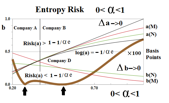
Figure 7.2: Entropy Risk
The “brown line” in the chart on the left, Figure 7.2, shows the minimum number of “basis points” that must be negotiated between the producer and the customer to “lift” the process out of the “blue box” in-process; “random events”, out-of-process, could, of course, be anything, but the systemic “profit” is negotiated in the “blue box”, in-process.
For example, on the right of the chart, at about b=0.6 and α near 1, there are about 60 basis points in the “blue box”, in-process.
If the points are not negotiated, or less than that, then the process will “end” at (a(M), b(M)) and “begin” production at (b(M), a(M)) with a(left)=b(M) and b=a(M), and the process will stay in the “basin”.
How much do you need?
We also note that log(a) = -1/αe < a(M) and a(N) < α, for all of Company B (1/e < α <1), which is a requirement that the “blue box” be entirely contained in the “edge of the wedge”; log(a) = -1/αe defines the left-hand side of the wedge and the modality, α, defines the right-hand side; please see Exhibit 6 above.
Things get a little bit “tight” as we approach the “death embrace” at Company D; however, the two “↑” up-arrows, near Company D, which are worth about five basis points, show that almost any “negotiation” between the producer and the customer will lift the producer out of the “blue box” and could even change the modality but that more is required at Company D.
For more details, please see our Posts “(P&I) The Process – The 1st Real Dollar” which shows how a “currency” gets its value from the “subsistence economy” at the Company D modality, and “(P&I) The Process – The Guns of August” which explains how that modality actually “works”.
For more applications of these concepts please see our Posts which rely on the Theory of the Firm developed by the author (Goetze 2006) which calibrates The Process to the units of the balance sheet and demonstrates the price of risk as the solution to a Nash Equilibrium between “risk-seeking” and “risk-averse” investors within the demonstrated societal norms of risk aversion and bargaining practice. And for more on The Process, please see our Posts The Food Chain and The Process End-Of-Process.
And for more information on real “risk management” and additional references to the theory and how to read the charts and tables, please see our Post, The RiskWerk Company Glossary; we’ve also profiled hundreds of companies in these Posts and the Search Box (upper right) might help you to find what you’re looking for.
And for more on what risk averse investing has done for us this year, please see our recent Posts on The S&P TSX “Hangdog” Market or The Wall Street Put or specialty markets such as The Dow Transports & Utilities or (B)(N) The Woods Are Burning, or for the real class action, La Dolce Vita – Let’s Do Prada! and It’s For You, Dear on the smartphone business.
And for more stocks at high prices, The World’s Most Talked About Stocks or Earnings Don’t Matter – NASDAQ 100. And for more on what’s Working in America, Big Oil, Shopping in America or Banking in America, to name just a few.
Postscript
We are The RiskWerk Company and care not a jot for mutual funds, hedge funds, “alternative investments”, the “risk/reward equation” and every other unprovable artifact of investment lore. We have just one product
The Perpetual Bond™
Alpha-smart with 100% Capital Safety and 100% Liquidity
Guaranteed
With No Fees and No Loads on Capital
For more information on RiskWerk, please follow the Tags or Categories attached to this Letter or simply enter Search for additional references to any term that we have used. Related data may be obtained from us for free in a machine readable format by request to RiskWerk@gmail.com.
Disclaimer
Investing in the bond and stock markets has become a highly regulated and litigious industry but despite that, there remains only one effective rule and that is caveat emptor or “buyer beware”. Nothing that we say should be construed by any person as advice or a recommendation to buy, sell, hold or avoid the common stock or bonds of any public company at any time for any purpose. That is the law and we fully support and respect that law and regulation in every jurisdiction without exception and without qualification to the best of our knowledge and ability. We can only tell you what we do and why we do it or have done it and we know nothing at all about the future or the future of stock prices of any company nor why they are what they are, now. The author retains all copyrights to his works in this blog and on this website. The Perpetual Bond®™ is a registered trademark and patented technology of The RiskWerk Company and RiskWerk Limited (“Company”) . The Canada Pension Bond®™ and The Medina Bond®™ are registered trademarks or trademarks of the Company as are the words and phrases “Alpha-smart”, “100% Capital Safety”, “100% Liquidity”, ”price of risk”, “risk price”, and the symbols “(B)”, “(N)” and N*.
