(P&I) The Process – End Of Process (E,C,D)

What time is it? Are we too early?

Essay. The system dynamics of The Process are rather “ordinary” and there is no sense that we are dealing with a “chaotic” or “turbulent” system, profane with “bubbles” or “black holes” or the “heat death”.

Nevertheless, if we can make a distinction by counting, at least in principle, in which entropy is conserved, then we are confronted with the 1st and 2nd E-conditions, a×log(a) = α×log(b) and b×log(b) = α×log (a), respectively, that also need to be respected, and the entropy of such a system is Ω(b) = -∫ b(a)×log(b(a))da = α and depends only on the modality, 0<α<+∞; please see our recent Post, “The Process – System Dynamics” for more information on this.

The most interesting events, from the point of view of system dynamics, occur at the “end-of-process” in which “payables” are exchanged for “receivables”, and for which the former are developed by the process in-process, and the latter are developed in the “trading connections”, who are also in-process, and which enable the process and are the reason for its existence.

However, the “end-of-process” depends on the modality, or entropy, of the system, and its behaviour is different for the different “companies” that are defined by that modality, and which we have called Company A (0<α<1/e), Company B (1/e<α<1), Company C (1<α), Company D (α=1/e), and Company E (α=1), and different again for “extreme α” in which α < γ/2e ≈ 0.1047236… where γ is the Euler–Mascheroni Constant γ=0.57721… .

Energy, Mass and Entropy The Entropy Increases But Mass And Energy Are Conserved As e/m=c²=1

In the absence of a “Conservation Law”, the process is actually quite a blast (and might appear to be so in the case of some conservation laws), and we can demonstrate that by examining, in more detail, from the point of view of system dynamics, the three “easiest” companies, Company E, C, and D.

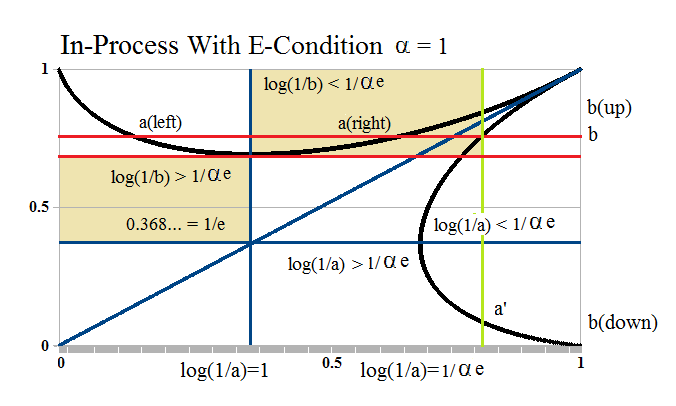
Figure 1: System Dynamics α =1

With reference to Figure 1 on the right (please click on it to make it larger if required), the two E-conditions, a×log(a) = α×log(b) and b×log(b) = α×log (a), divide the process-space into four regions corresponding to log(1/b) > 1/α×e and log(1/b) < 1/α×e, and log(1/a) > 1/α×e and log(1/a) < 1/α×e, respectively, where the first partition (of which we have shaded only a part) is determined by the 1st E-condition, a×log(a) = α×log(b), and that is a condition on (b) that is correct for all 0<a<1, in the “production space” of the process; and the second partition is determined by the 2nd E-condition, b×log(b) = α×log (a), and that is a condition on (a) that is correct for all 0<b<1, in the “production space” of the trading connections which we have mapped into the production space without any loss of information.

Since the process is in-process, we expect that sets of payables with a(left) = p((a(left)) < 1/e, will “implement” a progression from a(left) to a(right) with the “implementing set”, b=p((b)), for which a(left) and a(right) have the same measure, b, and, therefore, the same likelihood or probability of success, or occurrence, in-process, but for which a(right) is more “advanced” and closer to the end-of-process at a=b=1.

However, the implementing set (b) also defines a set (a’) with probability, a’=p((a’)), which is even more to the right of a(right), and a value of b=b(up) for a’ in-process, that is, it is on the 1st E-condition, and also b=b(down) which is an implementing set in the space of the “trading connections” for which b(down) × log(b(down)) = α×log(a’) and b(down)<b<b(up); please see Figure 1 above.

Moreover, b(up) at a’ then defines two new values of (a) in-process at a'(left)<a(left) < 1/e and a'(right) > a(right) >1/e, and b(up) > b > b(down), signifying the likelihood of even further progress towards the end-of-process.

Hence, beginning with any a(left) in-process, we can find an increasing sequence a(left)→a(right)→a'(right)→…→1 with the implementing sets b→b→b(up)→…→1, in the process receivables sets in the trading connections, and, concomitantly, a decreasing sequence a(left)→a'(left)→a”(left)→…→0 in the process space, with implementing sets, b→b(up)→…→1, and an increasing sequence, a(right)→a'(right)→a”(right)→…→1, in the process space of the trading connections, with implementing sets b→b(down)…→0, that is also in the process space of the trading connections.

The Never Ending End-Of-Process

A lot of motion, but no action.

As a consequence, the process never actually ends, because we never have a=b=1, in-process, but there is a continuing exchange of payables and receivables tending to an “end” at a=b=1, but it can never get there (please see below).

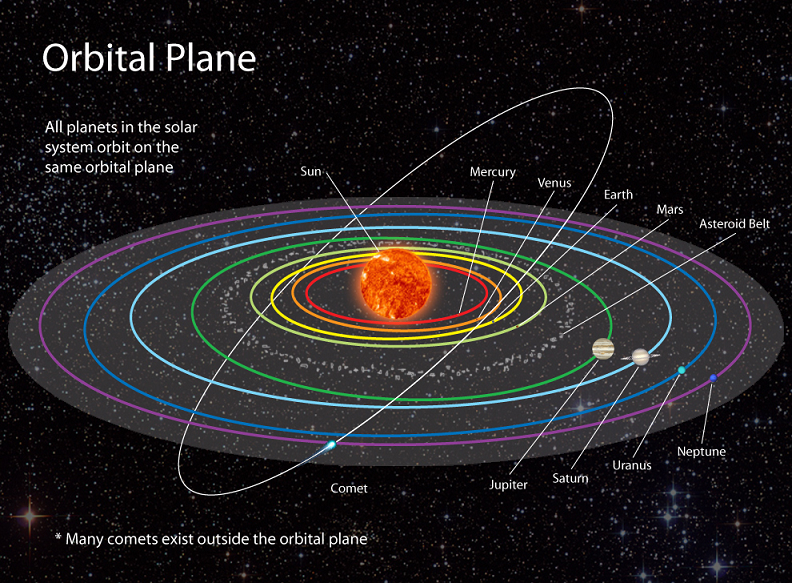
Nor does it mean that the exchange of payables and receivables is eventually too “small” to effect an “end”, or that there is nothing of significance that is happening; for example, our “solar system” is similar to the system dynamics of the process, in that there is a lot of motion, but only a small change in the system, over the eons.

We know, however, that “it” will end, and that it is only a small part and sub-process (or “company” with a small-“c”) of another “never ending” process, that will also end, and so on. But they never actually end in-process.

In summary, the “delivery of product” occurs at a=b=1, and the process in-process meets that burden with an increasing a(left)→a(right)→a'(right)→…→1 of payables sets, and an increasing b→b→b(up)→…→1 of receivables sets that are constrained by the 1st E-condition, a×log(a) = α×log(b).

And the trading connections prepare for the exchange, and a “receipt” of the “product”, with a similar b→b→b(up)→… tending to one, and set of payables a(right)→a’→…1 that are subject to the 2nd E-condition, b×log(b) = α×log(a).

However, it is important to note that the sets, styled as (a) and (b) with measures a=p((a)) and b=p((b)), and so forth, effecting each of the two E-conditions, are not expected to be the same, but only that they have the probabilities, or measures, that respect and implement the two E-conditions in-process; in fact, the two E-conditions have only two concurrent solutions, and those occur at a=b=1 and a=b=α, the modality; nor is it required, nor should we expect, that such sets, (a) and (b), should be the same in the latter; or even in the first, in which 1=p((a))=p((b))=p((N)), because they may always differ by sets of measure zero, which might not necessarily be of no consequence to the companies and people that are affected in-process; these events just don’t happen every day, so to speak, and could be likened to events such as a merger or acquisition, a break-through or break-down product, or an economic calamity, that may work to change the modality.

In addition to the sets (a,b) that tend to (1,1), there are necessarily also the sets (a(left), b(up)) that tend to (0,1) in the process space, and the sets (a’,b(down)) that tend to (1,0) in the trading connections, and it is these two sets, particularly a(left) and b(down), that “regulate” the progress of the process in-process to (1,1), and prevent the “explosion” that would otherwise occur at (1,1), should it ever get there; please see Figure 2 below.

With reference to Figure 1, all four sets can be engaged from the extreme case a(left)=a(right)=1/e and log(1/b)=1/α×e; the implementing set occurs at (a’,b) on the 2nd E-condition, which also results in the largest of the sets at (a'(left), b(up)) and the smallest of the sets at (a'(right), b(down)) with a'(right)=a’, as marked.

The “implementation” is demonstrated in the nine charts in Exhibit 1, below, which focus only on the events in the “corners” at (0,1), (1,1), and (1,0) and are correct for Company E and C, as illustrated, and each implementation starts at a(left)=a(right)=1/e, or, in the “natural coordinates” (please see below) of the process and the trading connections, 1=log(1/a); Company D is a little different (please see below), as are Company A and B, and the “corner” at (0,0) only comes into play for extreme α→0.

Exhibit 1: The Process From Different Points of View

Figure 2: E-Convergence (0,1)	Figure 3: E-Convergence (1,1)	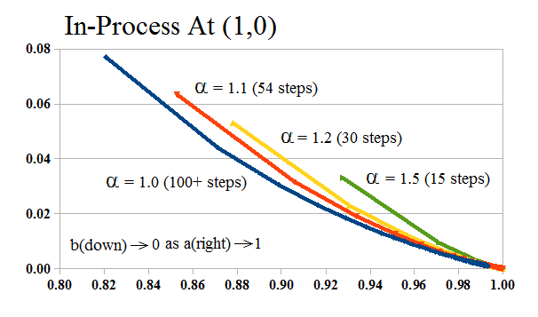Figure 4: E-Convergence (1,0)
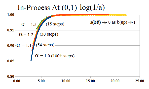Figure 5: E-Convergence (0,1) Log Scale (a)	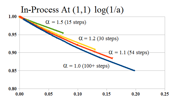Figure 6: E-Convergence (1,1) Log Scale (a)	Figure 7: E-Convergence (1,0) Log Scale (a)
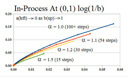Figure 8: E-Convergence (0,1) Log Scale (b)	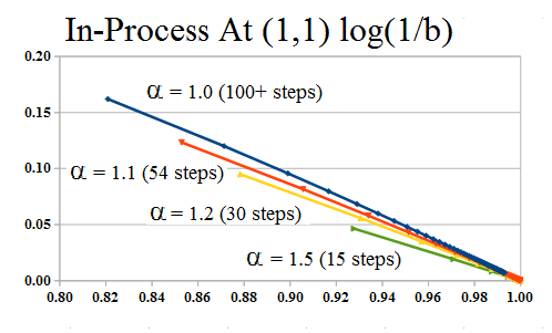Figure 9: E-Convergence (1,1) Log Scale (b)	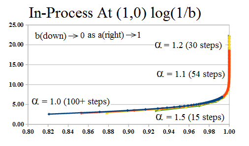Figure 10: E-Convergence (1,0) Log Scale (b)

In the absence of “time”, we have only “steps”, and each of these charts shows how many steps are required in order to get to within 1/1,000,000th (10^-6) of the “goal” from the same starting point, which is a=1/e and 1=log(1/a) in the “log scale”, or any a(left)<1/e would be just as good with one more “step”, or any a(right) with one less; please click on the charts to make them larger if required.

Which “one” are you?

These nine charts focus on the process from the point of view of the “producer” (or the process) and the “customer” which is the trading connections; the middle three charts show that there is “no problem” in the producer “producing” the product, and the customer “buying” it, both of which events demonstrate a high probability, and the same “number of steps” are required by both the producer and the customer in-process to get closer to the same unit (1) and effect the exchange, the producer “selling” it and the trading connections “buying” it, whatever “it” is.

However, nothing seems to be happening in most of the charts, but Figure 5 and Figure 10 look like “explosions”, and they are the number of “steps” that are required to get within a close tolerance of the end-of-process at (1,1), and that number decreases rapidly as the modality increases even slightly from α=1 to α=1.1, 1.2, and 1.5, in the natural co-ordinates of the process (Figure 5), and of the trading connections (Figure 11), but, thereafter, an “infinite” number of steps are required in each case in order to increase even further, and in all of that “time”, we’ve barely moved the needle, from a=1/e to a=10^-6 (1/millions) in so many steps, and then to 10^-9 (1/billions), and 10^-12 (1/trillions), and so forth, in orders of magnitude more.

Moreover, the beginning of it all, at a=0, b=1, progresses very rapidly towards the end of it all, at a=1, b=1, but will never get there, all the while spinning-off “profit”, which we will now collect; please see below.

The Capitalization Rate log(1/a)

These four charts show the same process as in Figure 1, above, but in the log(1/a)-scale; the “action” appears to be quite normal and realizable at (1,1), but we already know that’s not the case; moreover, the “action” goes-off to “infinity” at the beginning of process at (0,1), even as a→0 and b→1, which is better described as “comes from infinity” and “can’t go back” in-process, if we could look behind the “dot” at (0,1), and even more so, behind the “dot” at (0,0), both of which we’ll need to explain (sometime).

Exhibit 2: In-Process at (1,1) log (1/a) Far and Near

Figure 2.1: The Process in Log Scale 1st E-condition At (1,1)	Figure 2.2: The Process in Log Scale 1st E-condition
Figure 2.3: The Process in Log Scale 2nd E-condition At (1,1) in the process space	Figure 2.4: The Process in Log Scale 2nd E-condition in the process space

Charts like these are more familiar to physicists, chemists and biologists, but they’re also relevant to us, because log(1/a) is the “capitalization rate of 1 by a” (that is, 1 = a×exp(log(1/a))) and both of the charts Figure 2.2 and 2.4 show that the capitalization rate was enormous when the receivables sets, (b), had measures close to one and the payables sets, (a), had measures close to zero (right-hand side of Figure 2.2 and 2.4); then, dropped off to one at a=1/e with sets of measure 1/e=0.368… and continued to decrease to zero towards the end-of-process at a=b=1.

The capitalization rate is easily read-off from the charts in-process, because log(1/a) = -(1/α)×b×log(b) in process; for example, if b=0.75, then log(1/a) = -0.75×log(0.75) = 0.22 (22%), which is a high rate of “capitalization” and, in the parlance of “bonds”, would suggest that the asset was significantly under-priced if, in fact, it was worth (1) and would pay (1); the maximum capitalization rate always occurs at a=1/e, and it is 100%, and the capitalization rate of (b) is simply related to the capitalization rate of (a) by log(1/b) = (1/α)×a×log(1/a) = (1/α)×r×exp(-r), r=log(1/a), if (a) and (b) are in-process with modality α.

But, to put it yet another way, if the capitalization rate is low (<1), then the asset is riskier, and might not pay the (1) that we’re hoping for and, therefore, it’s an investment; a capitalization rate of  log(1/a)=1 (100%) means “cash”; and log(1/a)>1 (>100%) means “negative cash”, or less than “the” cash ($1) now, which is another way of tagging a currency devaluation.

Although it’s natural to think of the production as beginning at (0,1) and ending at (1,1), as in Figure 1, this analysis suggests that what actually happens is that the process emerges from the “death embrace” of Company D, at α=1/e, with a=b=1/e, and then moves on to either never-ending “production” at (1,1), or “receivership” at (0,1); that view is also supported by the Theory of Firm in which new companies are financed in the “N/B/W”-financing model as “40/60/25”, and the modality is α= 0.40 × (1-0.25) = 0.30.

Moreover, the capitalization rate is always 100% at a or b=1/e, and less thereafter, approaching zero at a=b=1 as “production” appears to be more and more of a certainty (Figure 2.1 and 2.3), and we need to wonder why it’s never zero, and the process never actually ends, but is always moving towards that goal.

The M- and N-Conditions & The Profit Motive

The End-Of-Process  The 1957 Cadillac & Ice Cream Cone

We proved in The Process that there are two necessary and sufficient conditions to effect the end-of-process without actually ending it, and we can describe that more colourfully as the “product”, which is sets of payables and receivables in-process, are “delivered” before the end-of-process in which the other product, such as cars and ice-cream cones, for example, are handed-over for cash, a payment and a receipt, and are, therefore, out-of-process, as well as out-of-pocket or out-of-plant, as the case may be.

The M-condition is pivotal to the “delivery of product” and the N-condition is pivotal to the “receipt of product” as (M-condition) 1+log(a) = lim (1/(b^α))×log(1+b^α), as b→0, and (N-condition) 1+log(a) = -lim (1/(b^α))×log(1-b^α), as b→0, and, as always, these are not the same a’s and b’s that effect the “limit”, which is notional in any case, but explains why “planned economies” will always fail, ever-reaching for the “limit”, but never getting there with a “product” that satisfies our aspirations for goods delivered with “profit”, and not just at par, which is signified by a=b=1.

To see this more clearly, we need to go into the “corners” at (0,1) and (1,0); please see Exhibit 3 below.

Exhibit 3: The End-of-Process In-Process

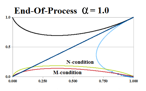Figure 3.1: End Of Process at (1,0) Alpha 1

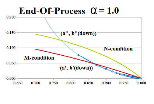Figure 3.1: End Of Process at (1,0)

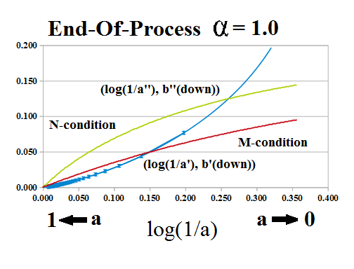Figure 3.3: End Of Process at (1,0) Log Scale

Figure 3.1 shows the “global picture” of the two E-conditions for α=1.0, and Figure 3.2 shows the “corner” at (1,0), or a=1 and b=0, with the “blue dots” showing the progress of a'(right) to 1 and b(down) to zero; Figure 3.3 is the same as Figure 3.2, but stated in capitalization terms as log(1/a). Moreover, the relations that are shown always obtain for any α, because both the M-condition and the N-condition are convex-down, and the 2nd E-condition (shown in “blue”) is convex-up near (1,0), and the difference for the same (a) and (b) is (1/(b^α))×log(1+b^α) + (1/(b^α))×log(1-b^α) = (1/(b^α))×log((1+b^α)×(1-b^α)) =  (1/(b^α))×log(1-(b^α)^2) <0 for any b>0 and any α>0; hence, for any b(down)→0, the corresponding a’ on the M-condition and a” on the N-condition, are such that a”<a'<1, and the capitalization rates are log(1/a’)<log(1/a”), as shown on Figure 3.3.

The “product”, which is “payables” and “receivables”, and not “payments” and “receipts”, can, therefore, be “delivered” in-process at (a”, b”(down)) on the N-condition, or at (a’, b'(down)) on the M-condition, and the relationships, or “decision factors” are a”<a’ and b”(down)>b'(down), and delivery “in-process” is demanded at (a’, b'(down)) in-process, which is the last chance to do so.

How much do you really want for this? May we suggest …

However, it may be advantageous, to “buy” the product with less cash and more receivables (or “credit”) at  (a”, b”(down)), should the producer so offer; moreover, there are “terms” that can be negotiated in-process between these two points, because the capitalization rate at (a”, b”(down)) is higher than the capitalization rate at (a’, b'(down)), which means that the “price for cash” (or the “producer price” or the “wholesale price” or the “warehouse price”, or even the “sale price”, if inventory is a problem) should be, or could be, lower at (a”, b”(down)) than at (a’, b'(down)).

Hence, an economy in which exchange is negotiable, and not demanded at par, will be an economy and not just a “dead process” absent of credit.

Company D In-Process

Welcome to the “Hotel California” – if we visit it, we can never leave without some help from our friends; please see Exhibit 4 below.

Exhibit 4: Company D In Process

If we are at (a,b) = (1/e, 1/e), then there are no implementing sets that will move us forward in-process; all we can do is enjoy the one we have, in perpetuity.

The relative position of the M-condition (shown in red) above the N-condition (green) at a=1/e and log(1/a)=1, also suggests, with respect to the 2nd E-condition in-process (shown in blue) that increasing the debt, and therefore, the payables, will command a higher capitalization rate, and will, therefore, be more expensive to the producer, and riskier for our “friends”, than if the reverse were true, as it is as a→1 at b(down); please see above.

However, should the company inspire such confidence, and raise the debt, then the advance to the end-of-process is quite rapid at a(right) and then to b(up), although the decline to receivership at a(left) is even faster if we decrease the payables (a) and increase the receivables (b).

For more applications of these concepts please see our Posts which rely on the Theory of the Firm developed by the author (Goetze 2006) which calibrates The Process to the units of the balance sheet and demonstrates the price of risk as the solution to a Nash Equilibrium between “risk-seeking” and “risk-averse” investors within the demonstrated societal norms of risk aversion and bargaining practice. And for more on The Process, please see our Posts The Food Chain and The Process End-Of-Process.

And for more information on real “risk management” and additional references to the theory and how to read the charts and tables, please see our Post, The RiskWerk Company Glossary; we’ve also profiled hundreds of companies in these Posts and the Search Box (upper right) might help you to find what you’re looking for.

And for more on what risk averse investing has done for us this year, please see our recent Posts on The S&P TSX “Hangdog” Market or The Wall Street Put or specialty markets such as The Dow Transports & Utilities or (B)(N) The Woods Are Burning, or for the real class action, La Dolce Vita – Let’s Do Prada! and It’s For You, Dear on the smartphone business.

And for more stocks at high prices, The World’s Most Talked About Stocks or Earnings Don’t Matter – NASDAQ 100. And for more on what’s Working in America, Big Oil, Shopping in America or Banking in America, to name just a few.

Postscript

We are The RiskWerk Company and care not a jot for mutual funds, hedge funds, “alternative investments”, the “risk/reward equation” and every other unprovable artifact of investment lore. We have just one product

The Perpetual Bond™
Alpha-smart with 100% Capital Safety and 100% Liquidity
Guaranteed
With No Fees and No Loads on Capital

For more information on RiskWerk, please follow the Tags or Categories attached to this Letter or simply enter Search for additional references to any term that we have used. Related data may be obtained from us for free in a machine readable format by request to RiskWerk@gmail.com.

Disclaimer

Investing in the bond and stock markets has become a highly regulated and litigious industry but despite that, there remains only one effective rule and that is caveat emptor or “buyer beware”. Nothing that we say should be construed by any person as advice or a recommendation to buy, sell, hold or avoid the common stock or bonds of any public company at any time for any purpose. That is the law and we fully support and respect that law and regulation in every jurisdiction without exception and without qualification to the best of our knowledge and ability. We can only tell you what we do and why we do it or have done it and we know nothing at all about the future or the future of stock prices of any company nor why they are what they are, now. The author retains all copyrights to his works in this blog and on this website. The Perpetual Bond®™ is a registered trademark and patented technology of The RiskWerk Company and RiskWerk Limited (“Company”) . The Canada Pension Bond®™ and The Medina Bond®™ are registered trademarks or trademarks of the Company as are the words and phrases “Alpha-smart”, “100% Capital Safety”, “100% Liquidity”, ”price of risk”, “risk price”, and the symbols “(B)”, “(N)” and N*.