(P&I) The Process – Debt & The Company We Keep

Mozart 1756-1791
Essay. “Debt” affects us all, and more than a few of our greatest artists have died in debt and rest (in pieces) in a pauper’s grave.
Countries tend to “forgive” each other, and vast billions are “vaporized” with the stroke of a pen, as being impossible, or pointless, to collect, in the hope that maybe we can do a more productive business another day.
Companies, too, are merely “fined” for infractions that would cripple we ordinary folk, and a company, or person, in “bankruptcy” is a sorry sight with not much left for the creditors they leave behind.
Do you know the difference between secured and unsecured debt?
The companies, organizations, and economies in Company A are the companies that we “keep”, so to speak, because they are all in debt, with vast amounts owing that may exceed what is owed to them by multiples of 3× to 5×, or more, and we have to wonder what that is all about.
Whether the debt is “secured” or not secured, doesn’t really matter; the new owners will get some inventory that couldn’t be sold by the old owners, and some plant & equipment that didn’t work for the old owners, and the shareholders will get nothing.
It is well-said that if we lend a person or company or government too much money, it becomes unclear who the “debtor” is, or will be.
Some of our largest debtors are governments and, after governments, sovereign wealth funds, public and private pension plans, and endowment funds of all sorts – they are in debt because the money is not theirs and they owe it to somebody, but can they pay, even if they want to?
And that’s a situation that affects many pension plans and endowment funds, now, because they do not or cannot “deliver” on their “unsecured promises”, and their “customers”, who have financed these “payables” for all these years, will need to “finance” them again in the years-to-come.

Dead in Twenty Years At +10%
For example, the Canada Pension Plan currently has invested assets of $200 billion, which are expected to increase to $800 billion in twenty years, and the multi-trillions thereafter.
But under its current mortality and employment assumptions, the plan is “dead” in twenty years if it tries to raise the benefits by just 10%; please see our Post “The Pensionnaires” for more information.

A “Banking Crisis”, you say?
Moreover, most persons, and countries, “live” in the “death embrace” of Company D with modality α=1/e, and that result is exactly a result of “the societal standards of risk aversion and bargaining practice”, of which either element – risk aversion or bargaining practice – can change from time-to-time, for a time, but not a long time, by declaration or opportunism, and leave behind a catastrophe of too much debt, or too little debt, which is also hard to bear for those of us who don’t have any money; please see our Posts “(P&I) – The End of Process (E,C,D)” and “(P&I) The Process – The Guns of August” for more information.

Do we have enough?
But despite all of this “debt trauma”, the “worth” of the dollar is forged in the cauldron of the “death embrace” of Company D, and it is kept there by the “balanced budget”, which is a budget of underdevelopment and underemployment and, in the absence of debt, we have only the “ownership society” in which all investments are funded by equity, or by “force” if there is not enough “equity” to go around; please see our Posts “(P&I) The Process – The 1st Real Dollar” and “(P&I) The Process – The Balanced Budget” for more information.
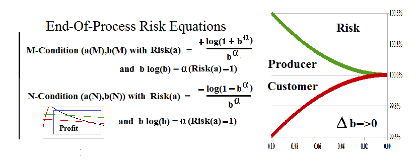
Figure 1: The Real Risk Equations
Nevertheless, we’re not complaining – we understand all of this perfectly – and there is a solution if there is a “problem” that wants for a solution; please see Figure 1 on the left, “The Real Risk Equations”, which we have previously developed in “(P&I) The Process – The WalMart Company B Story“, and which we’ll now apply to Company A, which are all in debt.

So, where do you live?
And we shall also see that “business” is done in Company B, C, and E, but “life” is “done” in Company D and Company A if we admit governments and pension plans, and many consumers, if not most, who are living beyond their means; please see below for more … on “life” and how it ends in debt.
A Life In Debt
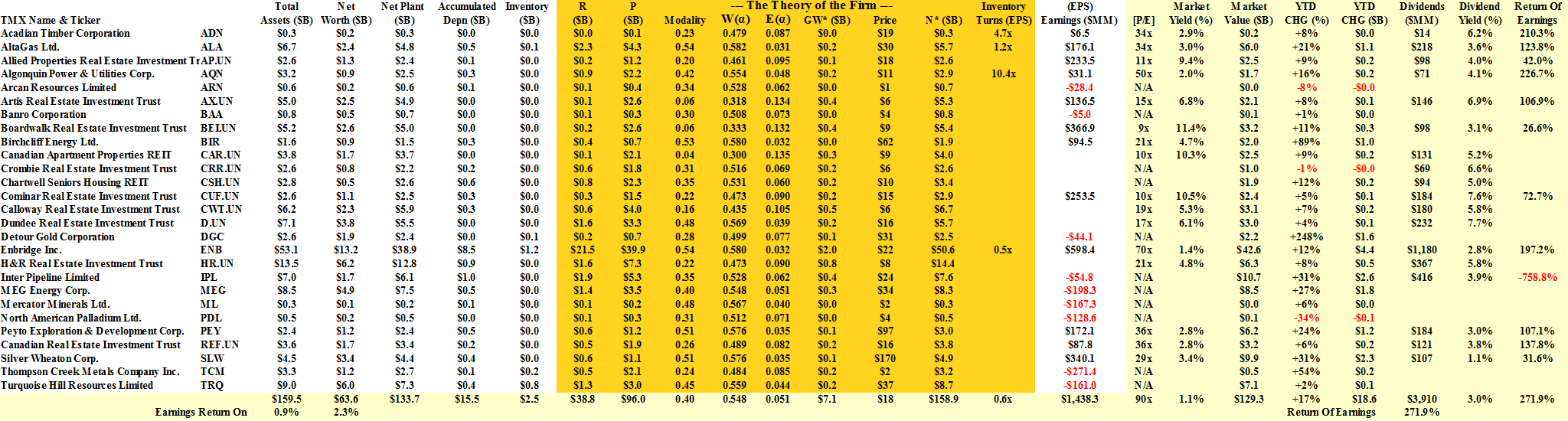
There are no Company A’s in the Dow companies (the industrials, transports, and utilities), but there is a lot of debt ($6.5 trillion), which exceeds their market capitalization ($5.8 trillion) even at the elevated prices of the past two years, and it also exceeds their net worth ($2 trillion) and even what they “own”, their fixed assets ($1.8 trillion) and their inventories ($2.5 billion), three-fold, so we can’t say that the debt is, somehow, “secured” by what they own, or less significant in their “big picture” than it is to a Company A; please see Exhibit 1 below for more details.
These companies are, however, “winding up” (upwards) because their “intrinsic net worth” (N*) is $3.6 trillion and 80% above their current net worth ($2 trillion) which means that if they keep on doing what they’re doing, day-in and day-out, Monday through Friday, then that relation will always obtain and appears to be very productive; please see our recent Post “(P&I) The Process – The WalMart Company B Story” for a longer explanation of these concepts.
There are, however, a few Company A’s in the S&P 500 NYSE (9 companies), the NASDAQ (4 companies), and the S&P TSX (27 companies) with an aggregate debt of $215 billion, which is less than 4% of the Dow debt, and these companies are also “winding up”, upwards aggressively, because their current net worth ($113 billion) is only a third of their intrinsic net worth (N*) at $324 billion; please see Exhibit 1 below for a summary and click on the links above for examples of Company A which, in general, could be a “company” or a government or a whole economy, and the only requirement is that they demonstrate a modality α, 0<α<1/e = 0.368… .
Exhibit 1: Debt & Its Fundamentals

All Market Fundamentals
The primary difference between the Company A’s, and Company D,and the others (Company B, E, and C), is that they “owe” (P) more than three times “what is owed to them” (R).
“What is owed to them” is (R), the sum of their total assets and accumulated depreciation, less “what they own” (their inventories and fixed assets), and since the debt (P) is also a substantial component of the total assets, as above, in aggregate and in both cases, the difference between the accumulated depreciation and their inventories and fixed assets, is pivotal in determining whether a company is a Company A with modality α=R/P < 1/e =0.368… or a Company B, E, or C; moreover, the “break point” occurs at Company D, α=1/e, which is at the top-end of Company A (0<α<1/e) and the low-end of Company B (1/e<α<1).
For example, in the case of the Dow companies, the accumulated depreciation is $1.3 trillion and the fixed assets are $1.8 trillion with inventories of $246 billion, whereas in the Company A’s, the accumulated depreciation is only $33 billion compared with fixed assets of $262 billion and an inventory of $14 billion; in percentage terms, that is 65% ($1.3 trillion/($1.8 trillion + $246 billion)) in the Dow companies, and only 12% ($33 billion/($262 billion + $14 billion)) in the Company A’s.
Not surprisingly, new companies are generally formed as Company A’s (please see the “60/40/25”-financing model of The Theory of the Firm); consumers are often Company A’s (“(P&I) The Process – The Balanced Budget“); and governments are usually Company A’s because their liabilities tend to grow faster than their “production”; and pension plans and endowment funds can be expected to be Company A’s, which is “bad news” for their owners and sponsors.
We also note that “accumulated depreciation”, “inventories” and “fixed assets” are concepts in this context, and accountants might need to look at it differently; but we’re concerned only with what these quantities have to do with the “business” of the company, as represented by (R) and (P), and although “taxes” are important, their effect shows up in the earnings and net worth, and we don’t need to know the details.
Debt & How It Ends
The production mode, and the “profit” of it, in-process, are decided in the “blue box” at the “end-of-production”, absent some “random” event that is out-of-process, but not necessarily insignificant or unlikely to occur again, such as “windfall-profits” or end-of-season inventory “clearance sales”; please see Exhbit 2 below for a “review” of the Company E and C modality, the Company B modality, and the Company D modality, and our previous Posts for more details.
The “blue box” is not quite a rectangle but it is determined by the modality, α, and the extreme extension of the 2nd E-condition, b×log b = α×log a, which occurs at log(a) = -1/αe (where “e” is the exponential) and where, as usual, a=p((a)) is the measure of a set of payables that are in-process with the set of receivables, (b), and, secondly, the intersection of the 2nd E-condition with the two end-of-process M- and N-conditions that affect the “customer” (the trading connections) and the “producer” at the end-process as Δb→0 and Δa→0, respectively.
Exhibit 2: The Risk Appetite
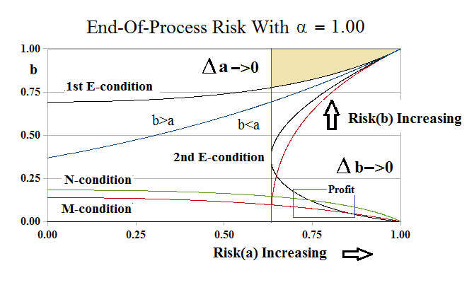 Figure 2.1: End-Of-Process Company E and C |
 Figure 2.2: End-Of-Process Company B |
 Figure 2.3: End-Of-Process Company D |
These charts of the 1st and 2nd E-conditions are rendered in the “risk co-ordinates”, Risk(a)=1+log(a), on the horizontal axis, for a=p((a)), the measure (or “probability”) of a set of payables, (a) of the process, and b=p((b)), on the vertical axis, for the corresponding set of “receivables” in-process with (a).
In these co-ordinates, “positive risk” is “bad” and a “burden” or a “load to bear”, and “negative risk” is “good” and can be thought of as an “investment” with a certain (probability one) outcome of success in-process.
To see this, we note that, 1=a×exp(log(1/a)), and if we set r=log(1/a), then “r” is the “capitalization rate” of (1) from (a), 1=a×exp(r), where, in fact, we are thinking about the aforementioned sets, (1) and (a), and their probabilities, 1=p((1)) and a=p((a)), in our usual notation and, therefore, 0=log(a) + r, and Risk(a) = 1 + log(a) = 1-r, and 1 = a×exp(1-Risk(a)) = a×e×exp(-Risk(a)).
Hence, if Risk(a)>0, then the capitalization rate of (1) by (a) is less than one and (a) is trading at a “premium” to (1) and will be “discounted” at the end-of-process; on the hand, if Risk(a)<0, then r>1 and (a) is trading at a discount to the unit, (1), meaning that (a) is an “investment” with a certain (probability one) outcome of (1), in this context.

More help for the “risk appetite”.
Another way to see this is that 1 = a×exp(r) = a×exp(1-Risk(a)) = a×e×exp(-Risk(a)); hence, if 1+i=exp(-Risk(a)), then 1=a×e×(1+i) and i<0 if Risk(a)>0, and i>0 if Risk(a)<0; hence, “positive risk” is “bad” and subject to an “expectation”, and “negative risk” is “good” and the break-point is at modality α=1/e if a=p((a)) is the measure of the total debt.
In this context, since the debt is largely “unsecured”, we can think of the debt not only as something that the producer “owes”, but also as something that the producer “owns” and obtaining “negative risk” on what we own is very difficult because it needs to made “productive” in order to accumulate to (1).
For example, WalMart Stores Incorporated has a ratio of 0.4× in its “earnings to inventory” (earnings $16 billion and inventory $42 billion) and its risk of the inventory is negative if that ratio is reduced to below 1/e=0.368… and the same ratio with respect to its “fixed assets” ($116 billion) is only 0.13× = $16 billion/$116 billion and it has, therefore, a “negative risk” with respect to its fixed assets and an almost negative risk with respect to its inventory.
In contrast, the Boeing Company has a hugely negative risk with respect to its inventory (0.103× = $4.2 billion/$41 billion, akin to “extreme alpha” with α<0.15 which we will discuss below) and positive risk (0.425× = $4.2 billion/$10 billion) for its fixed assets.

Maybe you can make it work?
In practice, then, obtaining “negative risk” in production is hard work, but obtaining it in the debt market is not so hard, and often quite easy; a company that has “negative risk” with respect to its liabilities, or even its assets, can “afford” to write them off, and they often are “written-off”.
We also note that our concept of “risk” has nothing to do with “volatility”, which is just “noise” and “random” events that have nothing to do with the words that move us in our investments – safe, liquid, and hopeful – and which also have nothing to do with the “productivity” of assets such as the inventory or fixed assets that we own.
“Volatility” is not risk and investment models that chase it, such as the Capital Assets Pricing Model (CAPM) and Modern Portfolio Theory (MPT), should expect random results.
Figure 2.1 (above) shows that the end-of-process for Company E, and that of Company C is similar, but that the “basin” defined by the 1st E-condition is shallower and the “shaded” area is shorter, thinner, and more to the right; the entire process for “production” occurs in the “basin” and the end-of-process is decided in the shaded area within which the 2nd E-condition intersects the M-condition (red line at the bottom) and N-condition (green line at the bottom) in the “blue box”.
The M-condition defines the in-process set, (a), as occurring with probability, a=p((a)), such that Risk(a) = 1 + log(a) = lim (1/b^α)×log(1+b^α) as b→1 and Δb→0, in which an “excess” of receivables (Δb) is developed in the trading connections in order to effect the exchange at a=b=1, which is the end-of-process, although it never gets there in-process.
On the other hand, the N-condition defines the in-process set, (a), also occurring with probability, a, but not necessarily the same (a) as above, such that Risk(a) = 1 + log(a) = -lim (1/b^α)×log(1-b^α) as Δb→0 and a→1 and Δa→0, as above, and it defines the “deficiency” of product that needs to made-up in production in order to effect the exchange, pro rata, at a=b=1.
Figure 2.1, as are the others, is a “state diagram” because “time” does not occur in the process if it is in-process; in principle, the in-process sets, such as (a) and (b), are developed from countable (effectively, finite) sets of payables and receivables that an accountant might render, but to be in-process, they are “filled-out”, so to speak, in order to account for the effectively endless opportunities of hypothecation and credit that are afforded by payables and receivables in-process, affecting both the producer and the customer (the trading connections).
“Progress” towards the end-of-process is rapid and takes only a few steps, but then takes smaller and smaller steps as Δb→0 and Δa→0, with it, because the steps are not independent, but need to be done in-process in order to be correctly done; the steps are more visible in Figure 2.2 as the line of red-dots on the 2nd E-condition in the lower right corner, but also appear as a “smudge” in Figure 2.1 near (1,0); for examples, please see our Post “(P&I) The Process – End Of Process (E,C,D)“
On the other hand, the producer and the customer can negotiate “terms” in the “blue-box” that result in the delivery and receipt of “product”, some of which might be tangible such as a service, or an automobile, but which also leave payables and receivables in-process so that the process continues; that is, we’re not interested in the one-time unique “product”, which doesn’t exist in any case because all products generate payables and receivables, and require the development of the trading connections.
The end-of-process for Company B is similar, except that Company B can “produce” in either the “NR-basin” as marked, or above the basin in a way that is the same as Company E or C; please see our Post, “(P&I) The Process – The WalMart Company B Story” for more information (and another review of what we’ve just said).
Company D, however, is quite different and the difference will be extended into the end-of-process for Company A; please see Figure 3.1, below, which is the same as Figure 2.3 above.
Exhibit 3: End Of Process Company D α=1/e=0.368…
Figure 3.1: End-Of-Process Company D
In Company D, the NR-basin has shrunk to a single point, (0, 1/e), on the left-hand side, where we note that, 0=Risk(a)=1+log(a), implies that a=1/e, as well.
The producer always assumes a positive risk, Risk(a)>0 once the process has “advanced” past a=1/e, but in Company B, E, and C, the customer does not assume a positive risk, Risk(b)>0, until much “later” when the production, (a), has advanced to the red-line, “Risk(b) Increasing” in all three of these diagrams.
Nevertheless, negotiation of the end-of-process exchange, in-process, can still take place in the “blue triangle” which is shown in Figure 2.3 and 2.4, and which might affect the payables (a) and receivables (b) that are realized at the end-of-process, and we would recognize them as a (necessarily) countable set of decisions, in-process, with measure zero.
Absent such negotiation, the process is always in the “death embrace” of Company D at α=1/e, and payables and receivables are endlessly created and exchanged as “product”.
Negative Risk & End-Of-Process For Company A (0<α<1/e)
Exhibit 4: The End-Of-Process For Company A

Figure 4.1: End-Of-Process Company A Risk Co-ordinates α=0.25<1/e=0.368…
A modality of α=0.25<1/e=0.368… , as shown in Figure 4.1 on the left, means that the producer owes four times as much as is owed to him (or her), and what he owes is a real liability that needs to be serviced; moreover, the liabilities are included in his payables and the “customer” is among his creditors for his “payables” which are among their “receivables”.
It’s not surprising, then, that in order for our debtor, Company A, to remain in business, the trading connections have to take a more “active” role in this “venture” but, as we shall see below, there is a limit to what even the deep-pockets of the trading connections can do for this “venture” that is supposed to be operating at a low modality, α<1/e, which is defined by its “total liabilities” (P) against “what is owed to it” (R), α=R/P, and the same concept applies to other assets (such as the inventories or fixed assets, please see above) because excessive, unsecured, or even “secured”, debt is an “asset” to the producer.
We also note that Risk(a) is negative and, therefore, “good” for him, but Risk(b) for the “customer” is already positive, reflecting a need to not only “finance” the producer, but also to “pay for the product”, should it be produced, and that is a situation that minds us, once again, of the all too common “production” of today’s pension plans and endowment funds, once reserved only for “gold mines” on-the-hoof, and invariably represented with the same enthusiasm until reality sets in.
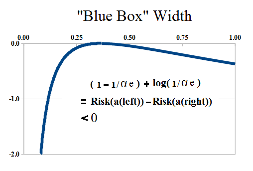
Figure 2: “Blue Box” Alpha
With reference to Figure 4.1, the “blue box” has gone “vertical” and the “NR-basin” has been “tipped-over”, 90º to the right, and extends upwards from the line through the intersection of the 2nd E-condition at b=α and, therefore, α×log(α) = α×log(a), on the right, which we may re-phrase as Risk(a) = 1 + log(α) = -log(1/αe), and to the left at b=1/e and Risk(a)=1-1/αe, and we note that the width of the in-process area now depends on the difference, (1-1/αe) + log(1/αe)<0, for all 0<α<1/e, and the difference becomes “quite large” as α→0; please see Figure 2 on the right.
The receivables sets, (b), affecting the customers (the M-condition, (M)), tend to be larger than the receivables sets affecting the producer (the N-condition, (N)) in the “negotiations” that might occur; for example, in Figure 3.1 above, b=b(M)=0.44 and b=b(N)=0.32, which means that b(M) is 38% more than b(N), although that situation reverses at “Extreme Alpha” less than α<γ/2e ≈ 0.1047236… where γ is the Euler–Mascheroni Constant γ=0.57721… ; please see The Process for more details.
Moreover, the payables set that the customers are negotiating will always tend to be higher than what the producer needs in-process; for example, in Figure 3.1 above, Risk(a(M)) =-0.448 and Risk(a(N)) =-0.455, so that the corresponding a(M) and a(N) values are a(M)=0.2351 and a(N)=0.2333, and a(M) is 1% more, and that difference increases as the modality decreases.
The customers, then, have a “conflict of interest” in that they want the product, but they also need to finance its production, whereas the producer appears to be “more relaxed” and might be prone to malingering even while in-process; to see how this plays-out as α→0, we have increased the relative liabilities through α=0.15 (6×), 0.10 (10×), and 0.05 (20×) in Figure 5.1 through Figure 5.3 below:
Exhibit 5: The End-Of-Process Risk For Company A
 Figure 5.1: End-Of-Process Company A Risk Co-ordinates Alpha=0.15 |
 Figure 5.2: End-Of-Process Company A Risk Co-ordinates Alpha=0.10 |
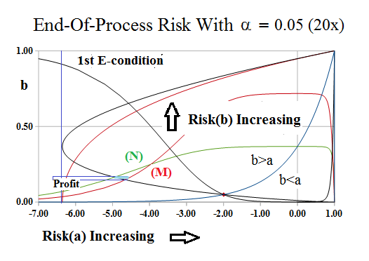 Figure 5.3: End-Of-Process Company A Risk Co-ordinates Alpha=0.05 |
Figure 5.1 is about as good as it gets for low modality; the producer “begins” production at a=α, on the right, and reduces his risk by reducing payables, (a), and increasing receivables, (b), and brings the production into the “profit box” in which he and the customer can negotiate a “price”; for example, the producer solution, (N), can be implemented with the same payables but less receivables than the “customer solution”, (M), thereby deceasing the “customer risk” which has been positive throughout, and remains positive until the end-of-production.
Figure 5.2 brings us into an entirely different space; production begins as a=α, but “jumps” into the profit box by reducing payables and increasing receivables; in practice, “production” is slower because the producer needs to “consume” the payables which is done in production but also by paying them, for which more receivables are required.
In Figure 5.3, we note that the “profit box” has become “paper thin” and it would, in practice, take a long time to produce it; the receivables in-process, (b), for that level of payables, (a), are shown in the 1st E-condition at the top of the chart; there are companies with substantial assets that function at these levels (please see the links above S&P 500 NYSE (9 companies), the NASDAQ (4 companies), and the S&P TSX (27 companies), such as REITS (Real Estate Investment Trusts) which are, basically, “paying themselves out” as dividends to their owners and shareholders, and other companies might have to sell assets to raise receivables, and so forth.
A Business Is A Customer
The twelve “vignettes” (or “bullets”) in Exhibit 6 below are all on the same scale in the risk co-ordinates, and they all have the same elements as Figure 5.1 through 5.3 above, but they are like a “moving picture” from diffuse and incoherent “payables” with modality, and hence “entropy”, near zero, α≈0, on the left, to Company D, on the right, which can be described as the emergence of the “1st real dollar”; its “coherence” is the direct result of increasing entropy, and its “de-coherence” is the direct result of decreasing entropy, and “time”, as we recognize it, only begins at Company D, and, obviously, “time” has a lot to do with the feasibility of debt service.
We have also shown the “flat space” that begins at Company E, α=1, and continues into Company C, α>1, which is where most companies exist today; as the modality increases and α→+∞, then the “flat space” on the right becomes the “flat line” which is another kind of “death” that results from too much money and not enough investment to sustain it.
Exhibit 6: Entropy Risk 0<α<1/e
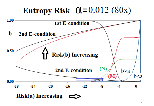 Figure 6.1 Extreme Alpha = 0.0120 |
 Figure 6.2: Extreme Alpha = 0.0130 |
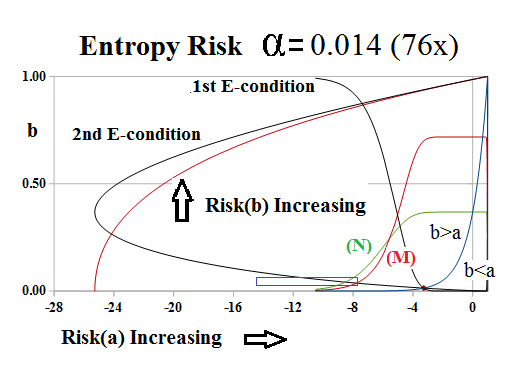 Figure 6.3: Extreme Alpha = 0.0140 |
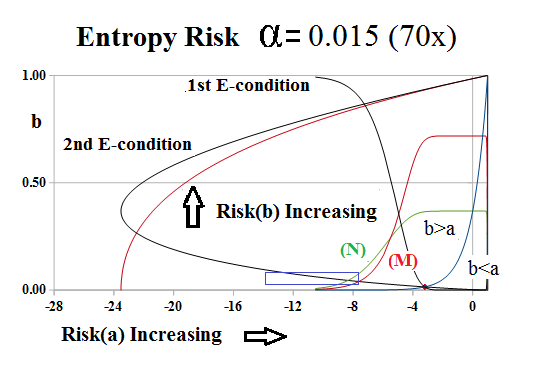 Figure 6.4: Extreme Alpha = 0.0150 |
In the first row, Figure 6.1 through 6.4, it would seem that nothing is happening and that nothing can happen between α=0 and α≈0.012, 0.013, 0.014, 0.015, and so forth; and that’s true, although we might wonder if (N)>(M) for all a=p((a))→0 and α→0 because there are four sets involved and not just two: the payables set, (a), that is being developed by the producer who has, already, a large “receivables” set, b=p((b)), that is defined by the 1st E-condition near the top of the charts, and similar sets for the customer, with b=p((b)) near zero in the “profit box” at the bottom of the chart.

Are You The One?
To answer the first question, we note that (N) has the “height”, -(1/b^α)×log(1-b^α)>0, for any a and b for which it is defined and in this case, for (a) near one in the producer space and (b) near one in the customer space; and similarly, (M) has the “height”, (1/b^α)×log(1+b^α)>0, for (b) in the customer space, with (b) near zero, and (a) in the producer space near zero, as Δa→0 and a→1 in the producer space, and Δb→0 and b→1 in the customer space; algebraically, (M) – (N) = (1/b^α)×[log(1+b^α) + log(1 – b^α)] = (1/b^α)×[log(1 – (b^α)^2)] <0, but that is not what is happening because the requisite a’s and b’s, in-process, are not the same, and we note, specifically, that the smallest value of (b) in the producer space occurs at a=1/e and it has the value log(b)=-1/αe from the 1st E-condition; please see below for more information.
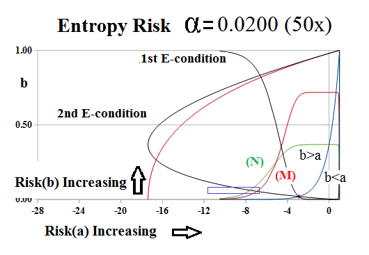 Figure 6.5: Extreme Alpha = 0.0200 |
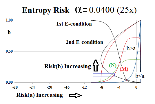 Figure 6.6: Extreme Alpha = 0.0400 |
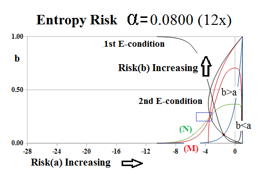 Figure 6.7: Extreme Alpha = 0.0800 |
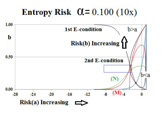 Figure 6.8: Extreme Alpha=0.100 |
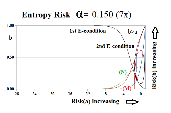 Exhibit 6.9: Extreme Alpha=0.150 |
 Figure 6.10: Extreme Alpha=0.250 |
 Figure 6.11: Extreme Alpha Company D |
 Figure 6.12: Extreme Alpha Company E |
With respect to these diagrams, we note that the producer function, the 1st E-condition, a×log(a) = α×log(b), hardly changes, and is a “constant” of the production in-process, and all of the “activity” is in the relationship between his production and the customer’s need for it, as demonstrated by being in-process with the 2nd E-condition, b×log(b) = α×log(a), for their sets of payables, (a), and receivables, (b).
Entropy Risk (0<α<+∞)
Entropy risk affects all assets and demonstrates the same properties as above; if it can be “capitalized”, then it has a modality and, therefore, an entropy. The case of the Boeing Company is a good example; the company is aggressively leveraged with debt which amounts to $86 billion in contrast to a net worth of $9 billion and its modality is α=0.68 which is the lowest of all the Dow Industrials.
“Debt” can be “destructive” if we are moving from right to left, both figuratively and “economically” or “socially”, as left- or right-oriented, and cases of “extreme debt” are relieved by debt forgiveness, as “uncollectable”, or by hyperinflation in the debt currency; or by default, and we note again that the producer has negative risk until near the end-of-production, but the customer has positive risk as soon as they are engaged at Risk(b)=0 (the red line in the above diagrams).
On the other hand, “debt” as diffuse and incoherent “payables” relative to the “receivables” at a low modality, is also “implosive” and creates the “1st real dollar”, moving from left to right, and the first (1).
The “event” at α=0 and a=b=0, on the extreme left, is not an “observable”; the reason is that the “behaviour” of the M- and N-conditions is “locally flat” as we increase the “precision” of our calculations, but “globally unpredictable” because the “size” of the variations, relative to each other, renders that “information” useless because we cannot comprehend that information in such a way that we might act on it.

Figure 3: Entropy Risk
The chart on the right, Figure 3, shows the one-step behaviour of the risk entropy near α=0, as the “blue box” defined by the 2nd E-condition and the M- and N-condtions, shrinks or expands as α→0.
For more details, please see our Posts “(P&I) The Process – The 1st Real Dollar” which shows how a “currency” gets its value from the “subsistence economy” at the Company D modality, and “(P&I) The Process – The Guns of August” which explains how that modality actually “works”.
For more applications of these concepts please see our Posts which rely on the Theory of the Firm developed by the author (Goetze 2006) which calibrates The Process to the units of the balance sheet and demonstrates the price of risk as the solution to a Nash Equilibrium between “risk-seeking” and “risk-averse” investors within the demonstrated societal norms of risk aversion and bargaining practice. And for more on The Process, please see our Posts The Food Chain and The Process End-Of-Process.
And for more information on real “risk management” and additional references to the theory and how to read the charts and tables, please see our Post, The RiskWerk Company Glossary; we’ve also profiled hundreds of companies in these Posts and the Search Box (upper right) might help you to find what you’re looking for.
And for more on what risk averse investing has done for us this year, please see our recent Posts on The S&P TSX “Hangdog” Market or The Wall Street Put or specialty markets such as The Dow Transports & Utilities or (B)(N) The Woods Are Burning, or for the real class action, La Dolce Vita – Let’s Do Prada! and It’s For You, Dear on the smartphone business.
And for more stocks at high prices, The World’s Most Talked About Stocks or Earnings Don’t Matter – NASDAQ 100. And for more on what’s Working in America, Big Oil, Shopping in America or Banking in America, to name just a few.
Postscript
We are The RiskWerk Company and care not a jot for mutual funds, hedge funds, “alternative investments”, the “risk/reward equation” and every other unprovable artifact of investment lore. We have just one product
The Perpetual Bond™
Alpha-smart with 100% Capital Safety and 100% Liquidity
Guaranteed
With No Fees and No Loads on Capital
For more information on RiskWerk, please follow the Tags or Categories attached to this Letter or simply enter Search for additional references to any term that we have used. Related data may be obtained from us for free in a machine readable format by request to RiskWerk@gmail.com.
Disclaimer
Investing in the bond and stock markets has become a highly regulated and litigious industry but despite that, there remains only one effective rule and that is caveat emptor or “buyer beware”. Nothing that we say should be construed by any person as advice or a recommendation to buy, sell, hold or avoid the common stock or bonds of any public company at any time for any purpose. That is the law and we fully support and respect that law and regulation in every jurisdiction without exception and without qualification to the best of our knowledge and ability. We can only tell you what we do and why we do it or have done it and we know nothing at all about the future or the future of stock prices of any company nor why they are what they are, now. The author retains all copyrights to his works in this blog and on this website. The Perpetual Bond®™ is a registered trademark and patented technology of The RiskWerk Company and RiskWerk Limited (“Company”) . The Canada Pension Bond®™ and The Medina Bond®™ are registered trademarks or trademarks of the Company as are the words and phrases “Alpha-smart”, “100% Capital Safety”, “100% Liquidity”, ”price of risk”, “risk price”, and the symbols “(B)”, “(N)” and N*.
