(P&I) The Process – In The Beginning

In The Beginning, Courtesy: The Studios

Essay. In the beginning, 1 million BC, there were no governments, corporations, banks, or taxes, and “governments” evolved long before corporations, banks, and taxes, and “corporations” long before banks and taxes, as we know them, although “taxes” and “tithes” or “duty”, have long been a part of our existence, with “services” more or less attached, but unlikely to be informed by our “vote”.

But there was “production” and, eventually, trade, and the economy that we consider in Figure 1.1, below, is already quite advanced (in fact, very advanced, as we shall see below) with an established modality of α=0.045 which means, roughly, that the “producer” owes only 20× as much as he (or she) is owed, suggesting that everything that was owed to him was no more than what he owned, and all of that was right in front of him, perhaps some stones and flint for making spearheads, for example, or straw for weaving baskets.

If, then, (a) is an arbitrary set of  “payables” and (b) is an arbitrary set of “receivables”, in the world, what is the probability, or likelihood, that they are in-process for some modality 0<α<+∞?

And the question could be phrased as “is there a business there”?

Since these are finite “sets” of “something” which is unit of  “currency”, and might just be “promises” of delivery, we can enumerate them, and if there are (k) payables and (l) receivables, and n=k+l, we can assign a “probability” of a=p((a))=k/n and b=p((b))=l/n, to each of them, and the question now becomes whether there exists an α, 0<α<+∞, such that these sets are in-process and, therefore, satisfy the 1st and 2nd E-conditions, a×log(a)=α×log(b) and b×log(b)=α×log(a), respectively.

Multiplying the first equation by (b) and the second by (a), a necessary condition for a solution is that b×a×log(a)=α×b×log(b) and a×b×log(b)=α×a×log(a), respectively, and substituting the 2nd E-condition in the right-hand side of the 1st equation, and the 1st E-condition in the right-hand side of the 2nd equation, we must have  that b×a×log(a)=α²×log(a) and a×b×log(b)=α²×log(b), respectively, for which there is the solution, α²=a×b, (and it’s unique) if and only if not both log(a) and log(b) are zero; that is, they are not both the entire “universe”, so to speak, for which a=b=1 (and, therefore, log(a)=0 and log(b)=0).

From this, we can conclude that if a=p((a)) and a=p((b)) are arbitrary numbers for which 0≤a,b≤1, the sets (a) and (b) are possibly in-process for some α, 0<α<+∞, only if a+b<2 and, therefore, in this case, that they are not the same sets, that is, that we can make a “distinction” between them.

To put it another way, if they’re different, there is a modality, but it might not be the one that we’re thinking of.

Enterprise Risk E(α)

With respect to the above example, we can (in theory) generate the σ-algebra, (N), with a Borel measure, μ, such that a=p((a))=∫χ(x∈(a))dμ(x), where χ(x∈(a)) = 1 if x∈(a) and zero otherwise; please see The Process for further details.

However, we can be certain that the probability measure, a=p((a)), is not the same discrete measure that we started with, although we can still ask the same question that if (a) and (b) are two sets in (N), are they in-process for some α, 0<α<+∞?

And the answer is the same, that (a) and (b) are in-process for some modality, α, if and only if log(a)+log(b)<0, but where we note that the set of payables, (a), are not necessarily payables that belong to one “company”, and the set of receivables, (b), are not necessarily a set of receivables that are developed in the trading connections of one “company”, but possibly many, and the issue is that if they are in-process for some α, 0<α<+∞, is there a “process” in (N), the σ-algebra that they generate,  that includes them?

Moreover, the sets (a) and (b) may differ from the whole space, for which μ(N)=1, by sets of measure zero, which could contain a countably infinite number of “decisions”, but they cannot have a common modality and, therefore, cannot be in-process with each other if both log(a)=0 and log(b)=0.

Which raises the practical question that if we are “auditors” or investors or regulators, for example, and we have some sets of payables and receivables, or just conclusions about them by some method, do they (really) belong to the “company” from which they purportedly came – that is, do they have the modality, α=R/P, which is demonstrated by their balance sheet, and for which, as usual, (R) is “what is owed to the firm”, net of “what it owns”, and (P) are its total liabilities?

And if not, what is it that we don’t know about the balance sheet, or about these “receivables” and “payables”?

The question is not trivial, or “academic”, because it’s easy to show, for example, that the banks are not what them seem; please see our recent Posts on “(P&I) The Banker’s Modality“, “(B)(N) The Canadian Bank Act“, and the “African Bank”, “(B)(N) ABL African Bank Investments Limited“, has never been a “bank” despite its pretensions to Tier 1, 2, and 3 “capital”.

To answer the question, we need to consider what sets, (a) and (b), demonstrate a “going-concern” and, therefore, will “deliver” the “product” at the end-of-process and, hopefully, that it is the same firm as the one that we’re thinking about.

For any modality, α, the “process space”, 0≤a,b≤1, which is the unit-square, can be mapped into the “risk space”, -∞<Risk(a), Risk(b)≤1, by a change of co-ordinates, as in Figure 1.1 below.

Exhibit 1: The Enterprise Risk Space

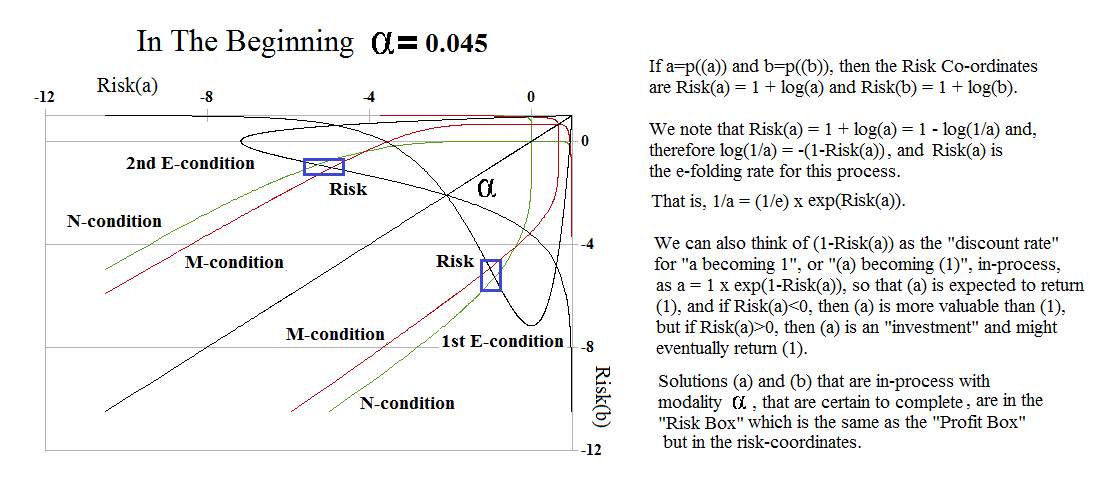
Figure 1.1: In The Beginning α-0.045

The “risk co-ordinates” for the probabilities, a=p((a)) and b=p((b)), are Risk(a) = 1 + log(a), and Risk(b) = 1 + log(b), so that log(1/a) = -(1-Risk(a)), for example, and 1/a=exp(-(1-Risk(a)) and Risk(a) is the “e-folding” rate which is familiar from “growth” and “decay” processes of all sorts in physics, chemistry, and biology.

That is, if r=Risk(a), then 1=a×exp(-(1-r))=a×(1/e)×exp(r), although we prefer to think of 1-Risk(a) as the “discount rate” of (a) with respect to (1) and that 1=a×exp(-(1-Risk(a)) with certainty if (a) is in-process with (b).

This becomes more colorful if we note that 1=a×e if and only if Risk(a)=0, which means that a=p((a))=1/e, and implies that if (b) is in-process with (a), then a×log(a) = α×log(b) and log(b)=-1/α×e, which is the lowest level of “receivables”, (b), that can occur in-process with (a).

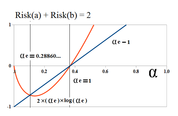
Figure 1.2: The Forbidden Fruit

Hence, Risk(a)+Risk(b) = 2+log(a)+log(b) ≤ 2, for all the sets, (a) and (b), whether or not they are in-process, and Risk(a)+Risk(b)=2 if and only if log(a) + log(b) = 0 which implies that if they are in-process (please see above), then a×b=α², for all a and b, 0≤a,b≤1.

In particular, when log(a)=log(1/e) and log(b)=-1/α×e, then log(a) + log(b) = 2×log(α) = -1 – 1/α×e <0, for which there are only two solutions – one of them is α×e=1, which is the Company D modality (α=1/e), and the other occurs at α ≈ γ/2e ≈ 0.1047236… where γ=0.57721… is the Euler–Mascheroni Constant and α×e≈0.28860…; please see Figure 1.2 on the right and The Process (Appendix) for the solution.

For these modalities, α=1/e and α≈ γ/2e ≈ 0.1047236…, there are always sets (a) and (b) in-process for which log(a)+log(b)<0, and if (a) and (b) are arbitrary sets in (N) for which we can, somehow, “cook the books” so that log(a)=1/e and log(b)=-1/α×e, then they are compatible, or consistent, with the process defined by either of these modalities.

But there are no others; please see Exhibit 2 below.

Exhibit 2: The Forbidden Fruit

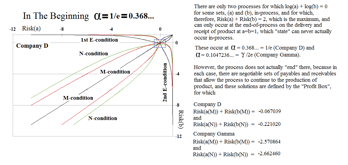Figure 2.1: In The Beginning – Company D

Figure 2.2: In The Beginning – Company Gamma

In these charts, there are always two “Profit Boxes” because we don’t know (in principle) whether the “producer” (payables)  is a customer (in the trading connections), or whether a “customer” (receivables) is the producer of the process which we are trying to find from our sample of payables (a) and receivables (b).

Company Gamma (Figure 2.2) is on the threshold of “extreme alpha” because, if he is the producer, then he owes about 10× (α=0.1047236) as much as is owed to him. As the modality decreases, the “process space” becomes nearly “empty”  and defines a “box” with co-ordinates (-∞,-∞) along the Risk(a)=Risk(b)-axis, ending at (1,1) in the upper-left corner, but the M-condition and N-condition end as “blunt objects” in the process space between (0,0) and (1,1); moreover, the behavior of these relationships is extraordinary between the “subsistence economy” at extreme alpha (beginning at α=0) to “more money than Croesus” at modalities α>2; please see Exhibit 4 below for some examples.

Exhibit 4: Unfolding the Modality, 0<α<+∞ – Modality Matters

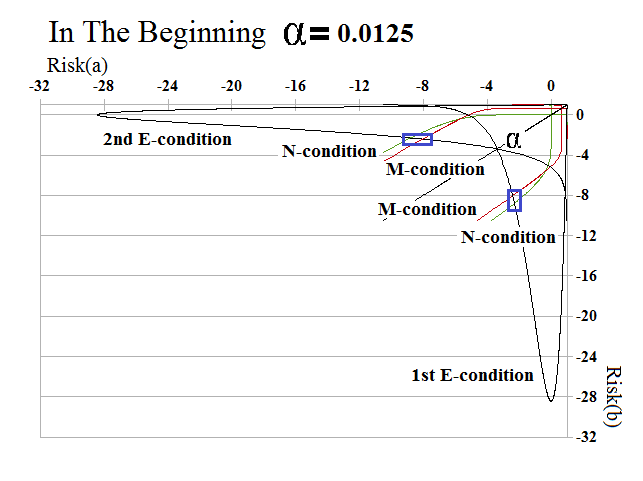Figure 4.1: In The Beginning Alpha=0.0125	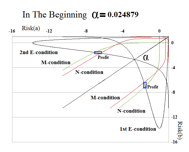Figure 4.2: In The Beginning Alpha=0.024879	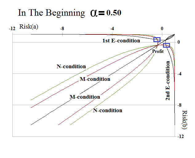Figure 4.3: In The Beginning Alpha=0.50
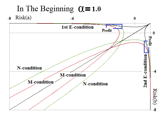Figure 4.4: In The Beginning Alpha=1.0	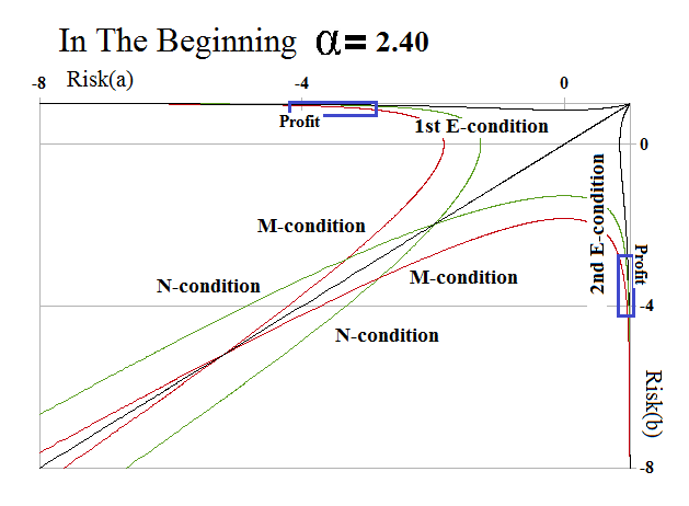Figure 4.5: In The Beginning Alpha=2.40	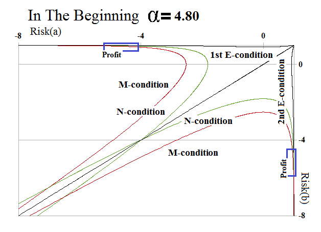Figure 4.6: In The Beginning Alpha=4.80

The 1st and 2nd E-conditions define the “process” that occurs in the production space of the “producer”, both with respect to his payables, and his receivables as they are developed in the production space of the trading connections which support his process and receive his product.

It’s implicit in the process – which makes a distinction between payables and receivables – that “his payables” (a) are not included in “his receivables” (b) because the only element that is both his payable and his receivable is “his cash”, and “cash” is not in-process, even though it could have positive effects on the balance sheet and influence other aspects of the process, such as credit or the working capital.

However, we are now considering arbitrary sets of payables (a) and receivables (b) in (N), and, in general, it is possible that (a)∩(b)≠Ø (the empty set); that is, for some company (or person) the set of payables (a) and receivables (b) contains an item – the same item – which is both his payable and his receivable and is, therefore, effectively “his cash” even though he might have written a “cheque” to himself, and it’s in the “float”, either directly or through some trading connections such as, for example, purchases and sales to his own companies, possibly at different prices, of which there are many examples, including the Enron Corporation, in its day.

But a=p((a)) and b=p((b)) are probabilities, and it is not true that p(((a)+(b)))=p((a)) + p((b)) unless (a)∩(b)=Ø (the empty set), where we will use the notation (a)+(b) for their union and (a)∩(b) for their intersection, and reserve (a)-(b) for the complement of (b) in (a).

Hence, even though a=p((a))=∫χ(x|x∈(a))dμ(x) and b=p((b))=∫χ(x|x∈(b))dμ(x), it is not true (in general) that a+b=∫χ(x|x∈(a)) + χ(x|x∈(b))dμ(x) = ∫χ(x|x∈(a)+(b))dμ(x) if (a)∩(b)≠Ø.

However, if it’s decided that such a “producer” is in-process, then the process modality, which is defined by ab=α² and, hence, log(a) + log(b) = 2×log(α), cannot be the same as that of his balance sheet, because log(a) + log(b) ≠ log((a)+(b)) (the union of (a)+(b)) if  “addition” is not correct; that is, a + b = ∫χ(x|x∈(b)-(a))×χ(x|x∈(a))dμ(x) is defined by the “convolution” of their probabilities and does not equal ∫χ(x|x∈(a)) + ∫χ(x|x∈(b))dμ(x) unless (a)∩(b)=Ø.

Figure 1.3: Enterprise Risk

Hence, we define the “Enterprise Risk” as, E(α) = 2×(1+log(α)), and it has the properties that E(α)<0 if α<1/e; E(α)=0 if α=1/e (Company D); and E(α)>0, α>1/e, with E(α)=2 if α=1 (Company E).

The Enterprise Risk, E(α), then defines a world in which “things add up” and we can “neatly” separate payables and receivables as “his” and “hers”, so to speak, and when things don’t add up, we might not have an “enterprise”, or it might not be the enterprise that we’re thinking about.

Based on the above, we might also expect that if (a) and (b) are in-process with modality, α, then Risk(a) + Risk(b) = 2+log(a)+log(b) = 2 + log(ab) = 2+2×log(α) = E(α), but that’s hardly ever true and it’s only asymptotically true as α→0, and as α→+∞; please Figure 1.3, on the right, and Exhibit 5 below.

The Enterprise Dividend

We define the “Enterprise Dividend” as the ratio, EM(α)/E(α), where EM(α) = Risk(a(M)) + Risk(b(M)) and (a(M),b(M)) is the default solution in the Profit Box at the end-of-process; please see our Post “(P&I) The Profit Box” for more information and background.

The Enterprise Dividend is similar to the pay-out rate of the “return of earnings” by dividends (please see our Post “(P&I) Dividend Risk & Dividend Yield” for more information) but, in this case, measures the return of cash and credit, by doing business and being in-process, over the cash and credit in a “perfect world” in which payables and receivables are endlessly exchanged, as “product”, and there is no “investment”, at either very low, or very high, modalities, so that, in effect, it’s a barter and subsistence economy regardless of its “wealth”.

The “nexus” is at Company D, α=1/e=0.368…, and it’s “positive” as the modality increases from low-levels to Company D, and “negative” if the modality decreases from higher levels, such as Company B to Company D; please see Figure 5.1 below.

Exhibit 5: Cash & Credit in the Real World – The Enterprise Dividend

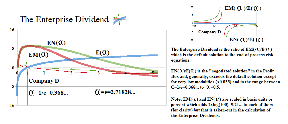
Figure 5.1: The Enterprise Dividend

The chart shows how economies develop, from the dark-ages of a subsistence economy at very low modality, even if such an economy is in-process, through the economies that we are more familiar with and which demonstrate a Company B, E, or C-modality.

On the other hand, an “asset-rich” economy, at modalities in excess of α>2, for which much more is owed to the producer (R) than what he owes (P), even net of what he owns, is not an “economy” at all – it’s more like a “kingdom” – and will wind-down and trade below the “perfect world” in the absence of investment that requires debt and engages the economy.

Are we in the Caves or Shangri-La?

From an investor or auditor or regulator point of view, however, we can easily calculate the modality of a company from its balance sheet, and if we have access to a catalog of its payables (P) and receivables (R), we can add them up, and expect that their ratio will be similar, at least qualitatively, to the modality that is represented by their balance sheet.

But if it’s not … we might have some work to do.

For more information and additional guides to the theory, please see our Posts “(P&I) The Process – The 1st Real Dollar” which shows how a “currency” gets its value from the “subsistence economy” at the Company D modality, and “(P&I) The Process – The Guns of August” which explains how that modality actually “works”.

For more applications of these concepts please see our Posts which rely on the Theory of the Firm developed by the author (Goetze 2006) which calibrates The Process to the units of the balance sheet and demonstrates the price of risk as the solution to a Nash Equilibrium between “risk-seeking” and “risk-averse” investors within the demonstrated societal norms of risk aversion and bargaining practice. And for more on The Process, please see our Posts The Food Chain and The Process End-Of-Process.

And for more information on real “risk management” and additioelownal references to the theory and how to read the charts and tables, please see our Post, The RiskWerk Company Glossary; we’ve also profiled hundreds of companies in these Posts and the Search Box (upper right) might help you to find what you’re looking for.

And for more on what risk averse investing has done for us this year, please see our recent Posts on The S&P TSX “Hangdog” Market or The Wall Street Put or specialty markets such as The Dow Transports & Utilities or (B)(N) The Woods Are Burning, or for the real class action, La Dolce Vita – Let’s Do Prada! and It’s For You, Dear on the smartphone business.

And for more stocks at high prices, The World’s Most Talked About Stocks or Earnings Don’t Matter – NASDAQ 100. And for more on what’s Working in America, Big Oil, Shopping in America or Banking in America, to name just a few.

Postscript

We are The RiskWerk Company and care not a jot for mutual funds, hedge funds, “alternative investments”, the “risk/reward equation” and every other unprovable artifact of investment lore. We have just one product

The Perpetual Bond™
Alpha-smart with 100% Capital Safety and 100% Liquidity
Guaranteed
With No Fees and No Loads on Capital

For more information on RiskWerk, please follow the Tags or Categories attached to this Letter or simply enter Search for additional references to any term that we have used. Related data may be obtained from us for free in a machine readable format by request to RiskWerk@gmail.com.

Disclaimer

Investing in the bond and stock markets has become a highly regulated and litigious industry but despite that, there remains only one effective rule and that is caveat emptor or “buyer beware”. Nothing that we say should be construed by any person as advice or a recommendation to buy, sell, hold or avoid the common stock or bonds of any public company at any time for any purpose. That is the law and we fully support and respect that law and regulation in every jurisdiction without exception and without qualification to the best of our knowledge and ability. We can only tell you what we do and why we do it or have done it and we know nothing at all about the future or the future of stock prices of any company nor why they are what they are, now. The author retains all copyrights to his works in this blog and on this website. The Perpetual Bond®™ is a registered trademark and patented technology of The RiskWerk Company and RiskWerk Limited (“Company”) . The Canada Pension Bond®™ and The Medina Bond®™ are registered trademarks or trademarks of the Company as are the words and phrases “Alpha-smart”, “100% Capital Safety”, “100% Liquidity”, ”price of risk”, “risk price”, and the symbols “(B)”, “(N)” and N*.