(P&I) The Process Extreme Alpha

Energy, Mass and Entropy The Entropy Increases But Mass And Energy Are Conserved As e/m=c²=1

Essay. It’s unlikely that a real company will acquire an extreme alpha but we still need to know that The Process is consistent at the “boundaries” as the modality α→0 or α→+∞ and that it doesn’t somehow “go off the rails” and surprise us if the modality decreases or increases outside of the normal range.

Moreover, The Process applies to any situation or complex in which there is a distinction that can be resolved by counting or selection and for which there is a “conservation law” of some sort; in the case of companies, we have R, P and the modality α=R/P which is implied by the balance sheet; but in the case of physical systems such as the energy and mass conservation that is implied by α=e/m=1=c² the “speed” of light in the right units we might expect that if it can happen, it will happen.

The Process Coupling At End-Of-Process

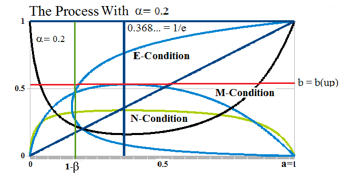
Figure 1: The Process Coupling At End-Of-Process

In The Process End-Of-Process the delivery and receipt of “product” at a=b=1 imposes conditions on the payables set (a) and receivables set (b) that require that each of them give up a “unit” (1) which they each must have and remain in-process during and after the exchange so that there is a new payables set (a) and a new receivables set (b) that satisfy the 1st and 2nd E-conditions after the delivery and receipt of product.

The necessary and sufficient condition that the trading connections can receive the product with those conditions is that there exist a set of receivables (b) in the (b)-space such that b=p((b)) and log(1+b)=Least Upper Bound {0<b<1|log(1+b)<(1/(1+b)^α)×log(1+(1+b)^α))} by the M-condition; and it is for such (b) that we also define the value of β=β(α)=b which is the value of β for which we calculate Arc(β,1) in the process space of the 1st E-condition and the “working capital” as W(α)=CR(α)-DB(α) with CR(α)=(1+β)-Arc(0,1) and DB(α)= β-Arc(β,1); please see Figure 1 above for the pre-delivery and pre-receipt conditions in which β=b is determined by the intersection of the 2nd E-condition and the M-condition in the (b)-space which we have mapped into the (a)-space as shown; however, it is the “length” b=β between (1-β) and 1 which is the measure of the receivables set required to complete the exchange that is significant in the (b)-space and it is the process length Arc(β,1) in-process in the (b)-space that is required to produce it.

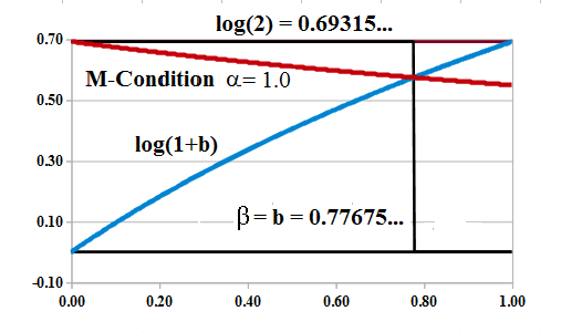
Figure 2: M-Condition Intersection α=1

With reference to Figure 2 on the right with modality α=1, it doesn’t seem like too much to ask that we can find such (b); the “blue line” is log(1+b), 0≤b≤1, and it is always the same for all 0<α<+∞ and monotonic increasing from zero to log(2)=0.69315….; the “red line” is (1/(1+b)^α)×log(1+(1+b)^α)) for the same 0≤b≤1 and it is monotonic decreasing from the value log(2) at b=0 to (1/2^α)×log(1+2^α) at b=1; therefore, all that we would have to show to prove the possible existence of such b=p((b)) is that (1/2^α)×log(1+2^α)<log(2) for all 0<α<+∞ because that would mean that the “red line” always starts above the “blue line” and always ends below it.

Figure 3: M-Condition Intersection α=30

However, the relationship becomes less evident in the case of extreme alpha; for example with reference to Figure 3 and 4 on the right, the 2nd E-condition b×log(b) = α×log(a) assures that there are sets (b) for b=p((b)) which assume both small values near zero and large values near one in a neighbourhood of a=1 which signifies the “completion of the product” or process at a=b=1 and these are required if α→+∞ (Figure 3) and α→0 (Figure 4).

Although the diagram in Figure 3 is compelling, it might be possible that the “red line” stays above the “blue line” and is tangent to it as α→0 and b→1; please see Figure 4 below.

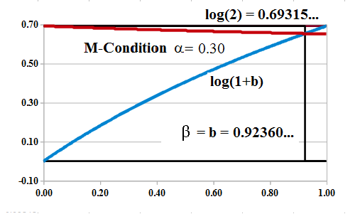
Figure 4: M-Condition Intersection α=0.30

To prove that (1/2^α)×log(1+2^α)<log(2) for all 0<α<+∞, we note that 2^α = 1 +h(α) where h(α) is strictly increasing from α=0 and h(0)=0 so that h(α)→0 as α→0; hence, we need to show that log(2+h(α))<(1+h(α))×log(2) which is equivalent to 2+h(α)<2^(1+h(α)) or that 1+h(α)/2 < 2^h(α); however, 2^h(α) = exp(log(2^h(α))) > 1+log(2^h(α)) = 1+log(2)×h(α)>1+h(α)/2 for all 0<h(α) and all 0<α<+∞; QED but we also note that the “restraint” is rather tight as α→0 and depends on the fact that (log(2) – 1/2)×h(α)>0 near α=0 even as h(α)→0.

The “production line” (shown as the “black line” in Figure 1 above) is defined by the 1st E-condition a×log(a)=α×log(b) and is strictly convex (upwards) for all α>0 which forces the relation Arc(0,1)→3 as α→0 and Arc(0,1)→1 as α→+∞.

To see this, we note that (1+log(a))=(α/b)×db/da where d/da is the derivative with respect to a and we apply it to the 1st E-condition; and therefore that d²b/da² =( (b/α)×1/a) + (1+log(a))×(1/α)×db/da=( (b/α)×1/a) + (1+log(a))²×(b/α²) > 0 for all 0<a<1 and 0<b<1 and shows that the 1st E-condition is strictly convex for all α>0; on the other hand, such b always obtains its minimum value at a=1/e so that log(b)=-1/(α×e)→-∞ as α→0 implying that b→0 as α→0; and log(b)→0 as α→+∞ implying that b→1 as α→+∞; since the production line also has the solution a=b=α and a→1 as b^α→1 with α→0 for any b, the production line “fills out” the entire boundary of the (a)-space as α→0 for the bottom and left- and right-hand sides; and the top (only) as α→+∞; hence, Arc(0,1) is monotonic increasing to 3 as α→0 and monotonic decreasing to 1 as α→+∞.

On the other hand, Arc(β,1)→0 as α→+∞ because β=β(α)→1 and both b→1 and Arc(0,1)→1 but Arc(β,1)→2 (not 3) as α→0; that is Arc(β=0,1)=2≠3=Arc(0,1) and the implication is that although a=0 is possible at the “start-of-process” for any α>0, β is formed in-process and can never be zero; please see Figure 4 above for α=0.30 and Figure 1 for the correct orientation of β in the process space; to prove this relationship, we know that the line which joins (0,1) to (β,b) with β×log(β) = α×log(b) is always inside the 1st E-condition (because it’s convex) and can therefore never be a part of Arc(β,1) in contrast to Arc(0,1) which tends to 3 and includes or “absorbs” the line as α→0.

Fra Luca de Pacioli, 15th century

The Modal Geometry of the Firm

There is presently no theory of the firm that ventures very far beyond the necessities and principles of the balance sheet, Total Assets = Net Worth + Total Liabilities; accounting theory, for example, explains the expenses and costs but not the benefit of the trading connections which can be calculated as the Coase Dividend and encompasses all of the elements of the firm including its assets and net worth and establishes a “common currency” that can be used to measure the “worth” and “future worth” of the enterprise that is represented and enabled by the firm.

For example, we can say that about half the companies in the Dow Jones Industrial Companies are “running-up” (and we know which ones they are) and about half of them are “running-down” and might want to take a look at what they’re doing day-in and day-out because what’s happening to them is built-in; and the same can be easily done within peer groups and entire industries such as the transports or the utilities; please see Exhibit 1 below.

Figure 5: The Modal Geometry of the Firm (21st Century)

The Theory of the Firm is an implementation of The Process in the context of the balance sheet and it can be explained in just a few charts that we call the “Modal Geometry of the Firm”; please Click on the chart to make it larger if required.

If we apply these concepts to the Dow Jones Industrial Companies, then the market “splits” into a group of companies that we have called the “Up-Winders” for those with (N*)>(N) and the “Down-Winders” for those with (N*)<(N); please see Exhibit 1 below.

Exhibit 1: The Dow Jones Industrial Companies – Fundamentals – April 2014

The Dow Jones Industrial Companies Up-Winders – Fundamentals – April 2014

The Dow Jones Industrial Companies Down-Winders – Fundamentals – April 2014

The Dow Jones Industrial Companies Up-Winders – Risk Price Chart – April 2014

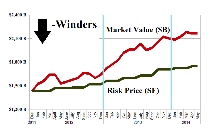
The Dow Jones Industrial Companies Down-Winders – Risk Price Chart – April 2014

At first glance there doesn’t seem much to distinguish these two groups of companies.

They both did well in the stock market last year with the Up-Winders gaining $405 billion and +18% and the Down-Winders gaining $460 billion and +26% even though there are fewer of them (16 Up and 14 Down); moreover, they have both tended to maintain those gains so far this year and are up +2% and +3% respectively.

The Up-Winders paid $77 billion in dividends to their shareholders last year for a return of earnings of 44% and an aggregate dividend yield of 2.9%; and the Down-Winders paid $56 billion for a return of earnings of 43% and an aggregate dividend yield of 2.6%; their [P/E]-multiples are also similar at 15× and 17× respectively; moreover, the equal-weighted cash-only Perpetual Bond™ held most of them most of the time (and all of them currently) and it returned +22% in the Up-Winders and +45% in the Down-Winders; please Click on the links (and again to make them larger if required) “The Dow Jones Industrial Companies Up-Winders – Prices & Portfolio – April 2014” and “The Dow Jones Industrial Companies Down-Winders – Prices & Portfolio – April 2014” for more of the details.

To see the difference, however, we need only look at the Risk Price Charts above; the market value of the Up-Winders appears to be consistently and substantially above their Risk Price (SF) whereas the Down-Winders seem to have suffered some misfortune in 2011 and 2012 and then exploded out-of-gate, so to speak, in the feverish buying of 2013.

Moreover, with reference to the tables in Exhibit 1, investors are willing to pay $32 for $1 of the Coase Dividend in the Up-Winders but only $20 for $1 of the Coase Dividend in the Down-Winders even though the Coase Dividend measures exactly the same thing in both cases; it measures the demonstrated ability of these companies to produce the values that are inherent in their balance sheets and the enterprise of their businesses.

The Up-Winders are in the enviable position of having their future net worth (N*) in the “float space” of the receivables and payables which they generate being greater than their current net worth (N) so that (N*)>(N) and they don’t have to change anything in order to earn it; all they have to do is stay in business and do the same business that they are always doing, day-in and day-out.

Indeed, first impressions are often the right ones.

The Down-Winders, however, have (N*)<(N) and they will have to work harder or smarter not to shrink and the price of the Coase Dividend is an aggregate assessment by investors of both that fact and the possibility that these companies will be or will not be effective; it’s probably for that reason that investors are so responsive and anxious to receive the most recent realized and forecast earnings reports for these companies, if not for all companies, although they generally don’t know the difference in quantitative terms or where the real battle actually is.

For more applications of these concepts please see our Posts which rely on the Theory of the Firm developed by the author (Goetze 2006) which calibrates The Process to the units of the balance sheet and demonstrates the price of risk as the solution to a Nash Equilibrium between “risk-seeking” and “risk-averse” investors within the demonstratedsocietal norms of risk aversion and bargaining practice. And for more on The Process, please see our Posts The Food Chain and The Process End-Of-Process.

Postscript

We are The RiskWerk Company and care not a jot for mutual funds, hedge funds, “alternative investments”, the “risk/reward equation” and every other unprovable artifact of investment lore. We have just one product

The Perpetual Bond™
Alpha-smart with 100% Capital Safety and 100% Liquidity
Guaranteed
With No Fees and No Loads on Capital

For more information on RiskWerk, please follow the Tags or Categories attached to this Letter or simply enter Search for additional references to any term that we have used. Related data may be obtained from us for free in a machine readable format by request to RiskWerk@gmail.com.

Disclaimer

Investing in the bond and stock markets has become a highly regulated and litigious industry but despite that, there remains only one effective rule and that is caveat emptor or “buyer beware”. Nothing that we say should be construed by any person as advice or a recommendation to buy, sell, hold or avoid the common stock or bonds of any public company at any time for any purpose. That is the law and we fully support and respect that law and regulation in every jurisdiction without exception and without qualification to the best of our knowledge and ability. We can only tell you what we do and why we do it or have done it and we know nothing at all about the future or the future of stock prices of any company nor why they are what they are, now. The author retains all copyrights to his works in this blog and on this website. The Perpetual Bond®™ is a registered trademark and patented technology of The RiskWerk Company and RiskWerk Limited (“Company”) . The Canada Pension Bond®™ and The Medina Bond®™ are registered trademarks or trademarks of the Company as are the words and phrases “Alpha-smart”, “100% Capital Safety”, “100% Liquidity”, ”price of risk”, “risk price”, and the symbols “(B)”, “(N)” and N*.